
Dolt is a version controlled SQL database; think Git and MySQL had a baby. Just over a year ago, we began our spatial journey with the addition of Spatial Types. We closed that gap about three months ago when we announced the support of Multi-Geometries. Now, we’re one step closer to full MySQL compatibility with support for Spatial Indexes…kinda.
What are Spatial Indexes?#
Spatial Indexes are a special type of Secondary Indexes that aims to improve the performance of spatial SQL queries like SELECT * FROM t WHERE ST_INTERSECTS(t.p, POINT(0, 0)).
Currently, this feature is only available after setting an environment variable; we’ll get into why later on.
export DOLT_ENABLE_SPATIAL_INDEX=1Here’s an example of how to create a SPATIAL index through the CREATE TABLE syntax:
tmp> CREATE TABLE tbl (p POINT SRID 0 NOT NULL, SPATIAL INDEX (p));
tmp> show create table tbl;
+-------+------------------------------------------------------------------+
| Table | Create Table                                                     |
+-------+------------------------------------------------------------------+
| tbl   | CREATE TABLE `tbl` (                                             |
|       |   `p` point NOT NULL SRID 0,                                     |
|       |   SPATIAL KEY `p` (`p`)                                          |
|       | ) ENGINE=InnoDB DEFAULT CHARSET=utf8mb4 COLLATE=utf8mb4_0900_bin |
+-------+------------------------------------------------------------------+
1 row in set (0.00 sec)
It’s also possible through the ALTER TABLE syntax if you already have a table with a GEOMETRY column:
tmp> CREATE TABLE tbl (p POINT SRID 0 NOT NULL);
tmp> ALTER TABLE tbl ADD SPATIAL INDEX (p);
tmp> show create table tbl;
+-------+------------------------------------------------------------------+
| Table | Create Table                                                     |
+-------+------------------------------------------------------------------+
| tbl   | CREATE TABLE `tbl` (                                             |
|       |   `p` point NOT NULL SRID 0,                                     |
|       |   SPATIAL KEY `p` (`p`)                                          |
|       | ) ENGINE=InnoDB DEFAULT CHARSET=utf8mb4 COLLATE=utf8mb4_0900_bin |
+-------+------------------------------------------------------------------+
1 row in set (0.00 sec)
SPATIAL indexes can only be defined over GEOMETRY columns (POINT, LINESTRING, POLYGON, etc.).
Additionally, SPATIAL indexes can only be defined over a single column and that column must have the constraints SRID and NOT NULL.
You can take advantage of SPATIAL indexes by filtering over certain Spatial Relation functions, like ST_INTERSECTS().
As of Dolt version v0.54.0, ST_INTERSECTS() is the only function that can take advantage of SPATIAL indexes.
You have to start somewhere. Over the next few weeks we will begin adding support for functions like ST_EQUALS(), ST_WITHIN(), etc.
Here’s an example:
tmp> INSERT INTO tbl VALUES (POINT(0,0)), (POINT(1,1));
Query OK, 2 rows affected (0.00 sec)

tmp> select count(*) from tbl where st_intersects(p, point(0,0));
+----------+
| count(*) |
+----------+
| 1        |
+----------+
1 row in set (0.01 sec)

tmp> explain select count(*) from tbl where st_intersects(p, point(0,0));
+---------------------------------------------+
| plan                                        |
+---------------------------------------------+
| GroupBy                                     |
|  ├─ SelectedExprs(COUNT(1))                 |
|  ├─ Grouping()                              |
|  └─ Filter                                  |
|      ├─ st_intersects(tbl.p,{0 0 0})        |
|      └─ IndexedTableAccess(tbl)             |
|          ├─ index: [tbl.p]                  |
|          ├─ filters: [{[{0 0 0}, {0 0 0}]}] |
|          └─ columns: [p]                    |
+---------------------------------------------+
9 rows in set (0.00 sec)
Under the Hood / A Deeper Dive#
Why Spatial Indexes? (Motivation)#
Let’s say we had a table with a million evenly spread out POINTs ranging anywhere from (0,0) to (1000, 1000), and we wanted to know how many points were in the region defined by POLYGON((0 0,1 0,1 1,0 1,0 0)).
So in SQL terms:
SELECT COUNT(*) FROM point_tbl WHERE ST_INTERSECTS(p, ST_GEOMFROMTEXT('POLYGON((0 0,1 0,1 1,0 1,0 0))'));Naively, to answer this query we’d have to call ST_INTERSECTS() for every POINT in point_tbl; that’s a million times we’re running the point-in-polygon algorithm.
Not to mention all the disk reads…
Logically, a POINT located far away from the origin (like (123, 456)) definitely does not spatially intersect with our POLYGON, so there’s no reason to run the expensive ST_INTERSECTS() function.
With a SPATIAL index, we’d be able to make these conclusions and avoid a great deal of unnecessary calculations.
How do Spatial Indexes work?#
Typically, indexes improve performance by neatly organizing the data into a B-Tree (in Dolt’s case a Prolly Tree).
However, POINTs don’t fit so neatly into this data structure, as they are multi-dimensional (they consist of two float64s x and y or latitude and longitude).
MySQL actually solves this problem by just not using a B-tree, and opting to represent their SPATIAL indexes as a R-tree.
While this does work pretty well, it isn’t without its drawbacks.
R-Trees are not deterministic; different insertion orders result in different trees with varying performance characteristics.
It’s possible to accidentally create highly unbalanced trees, degrading performance. Additionally, R-Trees’ non-determinism is not great for a versioned database that depends on maintaining history-independence.
For these very reasons, databases like Amazon Aurora and CockroachDB use a technique called Z-Ordering to map the two dimensional POINTs into one dimension and place them into a B-Tree/Prolly Tree.
They claim to achieve great performance benefits and avoid certain downsides, so Dolt’s going to do the same.
Specifically, Dolt requires history independence so we can merge Prolly trees.
Z-ordering is history independent so this technique fits the bill.
Z-Ordering#
As you might’ve guessed, it definitely matters how we perform this mapping.
An important factor is locality; we want POINTs that are spatially nearby to still be nearby after our mapping.
A simple, but ineffective mapping is to simply concatenate the bits x and y.
The mapping is quick to do, but does a terrible job of preserving locality.
Let’s say we’re dealing with small 3-bit integers, and see how this mapping pans out:
| x | y | concat | x_bits | y_bits | concat_bits |
|---|---|---|---|---|---|
| 0 | 0 | 0 | 000 | 000 | 000 000 |
| 0 | 1 | 1 | 000 | 001 | 000 001 |
| 1 | 0 | 8 | 001 | 000 | 001 000 |
| 1 | 1 | 9 | 010 | 000 | 001 001 |
Concatenating works pretty well in preserving the locality between (0, 0) , (0, 1), and (0, 2).
However, this pattern doesn’t hold for POINTs (0, 0), (1, 0), and (2, 0), as they are artificially far away.
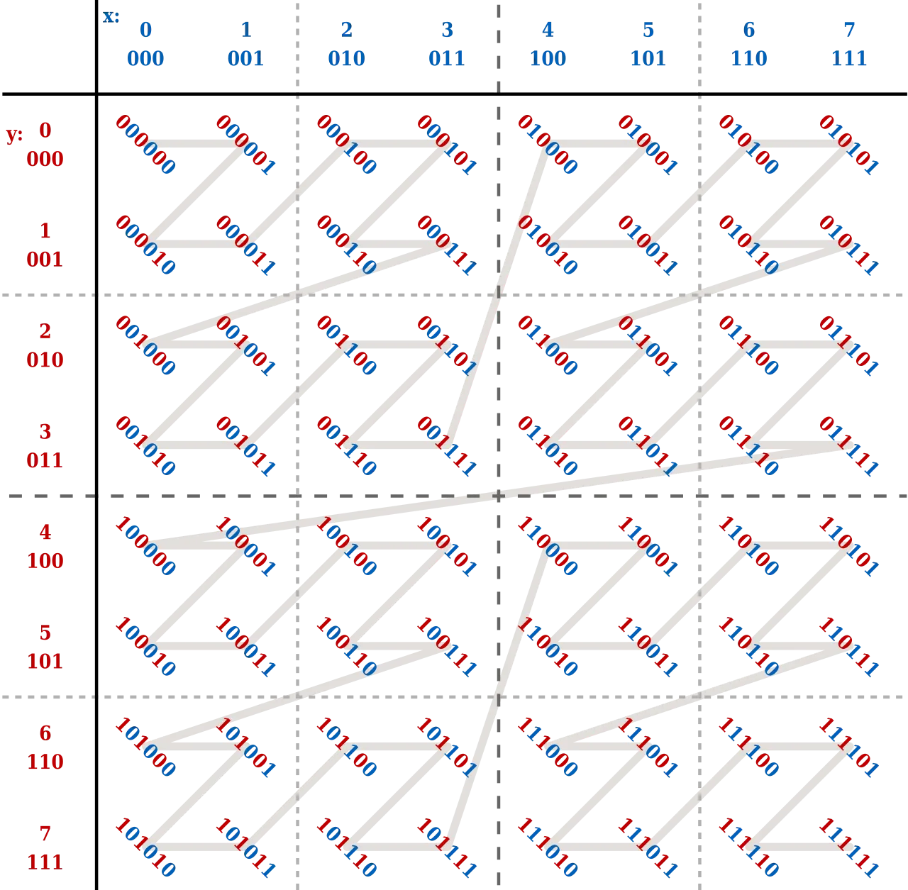
A relatively simple, but performant mapping is to use a Z-order curve.
It looks like this:
 I wonder where they got the name from…
Given two (or more) unsigned integers, we take their bits and interleave them. The resulting mapping is one-dimensional and maintains a high level of locality between our points; perfect for shoving into a B-tree.
| x | y | z_order | x_bits | y_bits | z_order_bits |
|---|---|---|---|---|---|
| 0 | 0 | 0 | 000 | 000 | 000 000 |
| 0 | 1 | 2 | 000 | 001 | 000 010 |
| 1 | 0 | 1 | 001 | 000 | 000 001 |
| 1 | 1 | 3 | 001 | 001 | 000 011 |
A Hilbert Curve is another space-filling curves that actually does a better job of spatial locality. However, due to the algorithm’s complexity and relatively expensive calculation, we stuck with Z-ordering.
Float Lexing#
You may have noticed that Z-Ordering works on unsigned integers, while we have signed floats.
They’re both 64 bits, but casting the raw bits of a float64 to a uint64 changes their ordering.
The signed bit is the first bit, so negative float64s reinterpreted as uint64s are larger than their positive counterparts.
So, we have to do another mapping; we want
-MaxFloat64to be close to00.0to be in the center, so0x80...0MaxFloat64to be close toMaxUInt64, so0xFF...F
Luckily, the IEEE-754 standard is amicable to this lexicographic remapping.
// LexFloat maps the float64 into an uint64 representation in lexicographical order
// For negative floats, we flip all the bits
// For non-negative floats, we flip the signed bit
func LexFloat(f float64) uint64 {
	b := math.Float64bits(f)
	if b>>63 == 1 {
		return ^b
	}
	return b ^ (1 << 63)
}
Dealing with Polygons#
Using float lexing and bit interleaving, we’re able to convert our POINTs into 16-byte Z-Addresses, ready to be placed into our Prolly Tree.
Well what about the other geometries, like LINESTRINGs and POLYGONs that contain multiple POINTs?
The trick is treating these geometries as POINTs and associating a size with them; we call these ZCells.
Without going into too much detail, this is the algorithm for creating ZCells:
- For a given geometry, find it’s bounding box, which consists of a
MinPoint(bottom left) and aMaxPoint(upper right). - Find the Z-Values of the minimum and maximum point,
zMinandzMax. - Find the matching prefix between
zMinandzMax; this is our level. - Create our Z-Cell, which looks like
[level_byte, z_0, z_1, ...].
Essentially, we’ve organized our geometries into 65 different levels. The larger the level, the larger the geometry; points are in level 0, and polygons that take up entire space are in level 64.
What do Spatial Index Lookups look like?#
Fortunately, our efforts to linearize the geometries so that they fit into the B-Tree makes creating lookups simple.
All SPATIAL index queries provide a GEOMETRY.
Using some logic from before, we can extract a bounding box from that GEOMETRY.
This is essentially a range of values to search over; they go from ZValue(minPoint) to ZValue(maxPoint).
Lastly, we prepend the level (creating 65 ranges) and (naively) perform this lookup in the same manner as a typical SECONDARY index.
Performance#
Finally, we’re able to read and write our geometries in an organized manner. So how much better is it? Well, here are some benchmarks:
| table | min_point | max_point | num_selected | select_% | keyless_sec | spatial_key | multiplier |
|---|---|---|---|---|---|---|---|
| point | (0, 0) | (0, 0) | 0 | 0 | 0.0761 | 0.0009 | 81.1x faster |
| point | (2, 2) | (4, 4) | 2 | 0.0004 | 0.1066 | 0.0009 | 109.4x faster |
| point | (2, 2) | (128, 128) | 2021 | 0.4042 | 0.1119 | 0.0325 | 3.4x faster |
| point | (2, 2) | (256, 256) | 8064 | 1.6128 | 0.1087 | 0.0542 | 2x faster |
| point | (2, 2) | (512, 512) | 32583 | 6.5166 | 0.1118 | 0.2109 | 1.8x slower |
| point | (0, 0) | (1000, 1000) | 124932 | 24.986 | 0.1121 | 0.2638 | 2.5x slower |
| point | (-1000, 0) | (1000, 1000) | 249152 | 49.830 | 0.1114 | 0.5167 | 5x slower |
| point | (-1000, 0) | (1000, 1000) | 382688 | 76.753 | 0.1139 | 0.9949 | 8.7x slower |
| point | (-2000, -2000) | (2000, 2000) | 500000 | 100 | 0.1128 | 1.0218 | 10x slower |
| point | (-1, -1) | (1, 1) | 0 | 0 | 0.1035 | 0.5115 | 5x slower |
| poly_1 | (0, 0) | (0, 0) | 0 | 0 | 0.0345 | 0.0011 | 29.3x faster |
| poly_1 | (2, 2) | (4, 4) | 0 | 0 | 0.0705 | 0.0013 | 53.4x faster |
| poly_1 | (2, 2) | (128, 128) | 383 | 0.383 | 0.0713 | 0.0060 | 11.7x faster |
| poly_1 | (2, 2) | (256, 256) | 1617 | 1.617 | 0.0742 | 0.0102 | 7.2x faster |
| poly_1 | (2, 2) | (512, 512) | 6503 | 6.503 | 0.0733 | 0.0356 | 2x faster |
| poly_1 | (0, 0) | (1000, 1000) | 25118 | 25.118 | 0.0705 | 0.0490 | 1.4x faster |
| poly_1 | (-1000, 0) | (1000, 1000) | 49862 | 49.862 | 0.0657 | 0.1055 | 1.7x slower |
| poly_1 | (-1000, 0) | (1000, 1000) | 76449 | 76.449 | 0.0614 | 0.1698 | 2.7x slower |
| poly_1 | (-2000, -2000) | (2000, 2000) | 100000 | 100 | 0.0597 | 0.2321 | 3.3x slower |
| poly_1 | (-1, -1) | (1, 1) | 1 | 0.001 | 0.0726 | 0.1264 | 1.7x slower |
The point table consists of 500,000 POINTs with random x and y values ranging anywhere from -1000 to 1000.
The poly_1 table consists of 100,000 randomly generated POLYGONs (triangles) whose vertices are all anywhere from 0-2 units apart.
Improvements#
When the query range is small enough, SPATIAL indexes significantly improve look ups.
For point table we see speedups from 80-100x, and for the poly_1 we see speedups from 10-50x.
Anti-Improvements#
However, when the selection ranges get larger, our performance drastically worsens.
In fact, in these cases it’s actually worse to use SPATIAL Indexes…about 2-10x worse.
Additionally, there’s even a degenerate case with the unit square POLYGON((-1 -1,-1 1,1 1,1 -1,-1 -1)); the actual selection range is relatively tiny, but has awful performance.
Here’s a graph plotting speedup multiplier against select percentage.
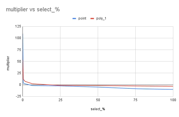
As you can see, there’s a quick drop off in performance when we start to query large portions of our data.
Future Work#
Evidently, there’s still a great deal of work to be done here.
Z-Range Pruning#
While the z-addresses preserve locality and do eliminate many spatial comparisons, a pass over the zMin to zMax still results in a ton of unnecessary comparisons.
Certain ranges around the “seams” or powers of 2 in the space of z-addresses, traverse over many z-addresses that are not within the original bounding box.
It is possible to break down these larger Z-Ranges into several smaller Z-Ranges using the LITMAX/BIGMIN algorithm. This is something we are currently working on.
Level Pruning#
For every range of Z-Values, we produce 65 more ranges, as there are 65 possible levels geometries could be in.
However, for tables like point, every POINT will be in level 0, yielding many unnecessary range searches.
Covering Indexes#
There is a performance distinction between covering and non-covering indexes.
Covering indexes can satisfy lookups with the key itself.
Meanwhile, non-covering indexes must perform another lookup to retrieve the value to satisfy the lookup.
This extra level of indirection leads to extra disk accesses, and subsequently worse performance.
Right now, SPATIAL indexes are strictly non-covering as their keys are bounding boxes, which do not have enough information to restore the full GEOMETRY.
Geometry Decomposition#
The S2 library performs something called Geometry Decomposition, which decomposes a GEOMETRY into the set of bounding boxes that efficiently contain it. Currently, we only create one large bounding box, which, depending on the GEOMETRY, may be too large.
Given the current state of their performance and the fact that implementing some of these optimizations may break compatibility between Dolt versions, SPATIAL indexes are behind the feature flag mentioned above. Good thing your database is versioned 😉.
Conclusion#
If you feel like experimenting, give SPATIAL indexes a try.
There are still some kinks to work out, but we are constantly improving and making Dolt better.
Remember we’re open source, and will gladly take public contributions.
Feel free to drop by on our Discord with any questions or feature requests!