
Dolt is the first relational database with history independent version control. Dolt’s Git-like commit graph captures snapshots in a format that efficiently diffs and merges tables and schemas.
We recently added index scan costing to Dolt’s SQL engine, go-mysql-server. Today we announce the latest improvements, statistics that survive server restarts and improve join costing.
Dolt users can opt into a preview of statistical join costing by running
ANALYZE TABLE <table> for join tables. This command collects and
stores histogram statistics for table indexes. Scans and joins whose
indexes have statistics automatically opt into finer-grained cost
estimates. We only support costing numerical comparisons. Queries
lacking a complete set of statistics necessary for estimation fall back
to our legacy costing heuristics. Automatic statistics refresh is coming
soon!
Intro#
The fastest way to preview statistics is to make a table with a some data:
create table horses (id int primary key, name varchar(10), key(name));
insert into horses select x, 'Steve' from (with recursive inputs(x) as (select 1 union select x+1 from inputs where x < 1000) select * from inputs) dt;
Our recursive common table expression inserts 1000 horses, all named Steve.
Then we analyze:
analyze table horses;The new dolt_statistics system table makes it easy to observe index
distributions:
select `index`, `position`, row_count, distinct_count, columns, upper_bound, upper_bound_cnt, mcv1 from dolt_statistics;
+---------+----------+-----------+----------------+----------+-------------+-----------------+-----------+
| index   | position | row_count | distinct_count | columns  | upper_bound | upper_bound_cnt | mcv1      |
+---------+----------+-----------+----------------+----------+-------------+-----------------+-----------+
| primary | 0        | 344       | 344            | ["id"]   | [344]       | 1               | [344]     |
| primary | 1        | 125       | 125            | ["id"]   | [469]       | 1               | [469]     |
| primary | 2        | 249       | 249            | ["id"]   | [718]       | 1               | [718]     |
| primary | 3        | 112       | 112            | ["id"]   | [830]       | 1               | [830]     |
| primary | 4        | 170       | 170            | ["id"]   | [1000]      | 1               | [1000]    |
| name    | 5        | 260       | 1              | ["name"] | ["Steve"]   | 260             | ["Steve"] |
| name    | 6        | 237       | 1              | ["name"] | ["Steve"]   | 237             | ["Steve"] |
| name    | 7        | 137       | 1              | ["name"] | ["Steve"]   | 137             | ["Steve"] |
| name    | 8        | 188       | 1              | ["name"] | ["Steve"]   | 188             | ["Steve"] |
| name    | 9        | 178       | 1              | ["name"] | ["Steve"]   | 178             | ["Steve"] |
+---------+----------+-----------+----------------+----------+-------------+-----------------+-----------+
The statistics summarize that the primary index, (id), increments from
1-1000 with all unique values. Even though the (name) index is also
divided between 5 buckets, each bucket only contains one distinct value,
'Steve'.
And that’s it! The SQL engine takes care of the hard part, using statistics to improve query plans.
Using Join Statistics#
We will walk through a more detailed example to show why statistics are useful and how they work!
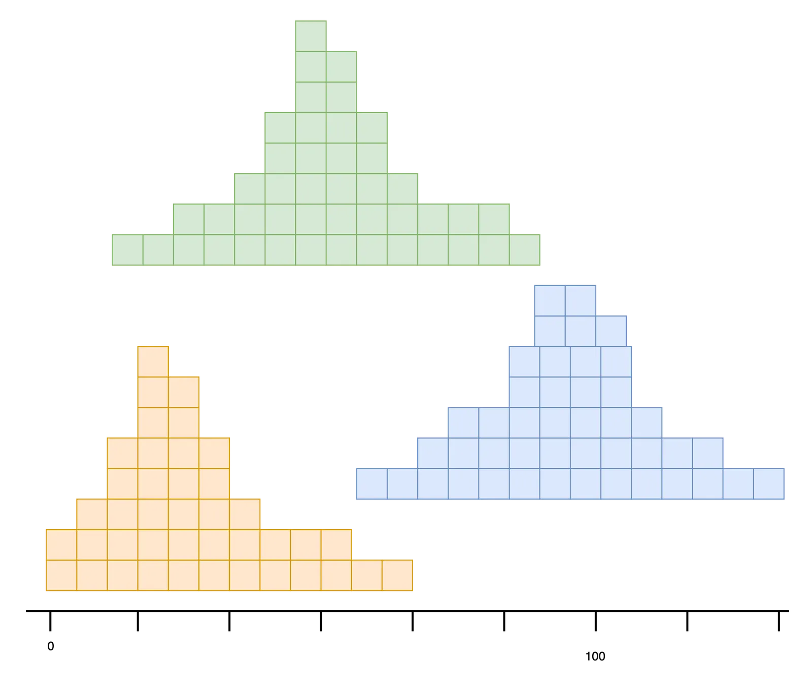
The focus will be a database of rainfall in different biospheres. The first table will include desert rainfalls, averaging 10cm of rain a year. The second table represents grasslands averaging 25cm of rain a year. And the third will represent deciduous forests averaging 100cm of rain.
Below is a representation of rainfall data generated by randomly sampling different normal distributions. The yearly values cluster around the associated mean but vary depending on the given year.
We will join the three tables to find years where the rainfalls overlap exactly. The output results represent three (maybe different) years where desert, grassland, and forest rainfalls are identical.
select d.rain, d.year as desert_year, g.year as grassland_year, f.year as forest_year
from desert d
join grassland g
  on d.rain = g.rain
join forest f
  on g.rain = f.rain;
We’ve blogged in the past about how the best join plan is usually constant complexity while the worst join plan is exponential, which in real time translates from ~milliseconds to ~years of latency for individual queries. For this reason it is important for our SQL engine to pick fast plans.
Our demo example is not so extreme, but the difference before (630ms)
and after (330ms) running analyze table desert, grassland, forest is
still noticeable in this toy example:
LookupJoin
 ├─ (d.rain = g.rain)
 ├─ MergeJoin
 │   ├─ cmp:(g.rain = f.rain)
 │   ├─ TableAlias(g)
 │   │   └─ IndexedTableAccess(grasslands)
 │   └─ TableAlias(f)
 │       └─ IndexedTableAccess(forest)
 └─ TableAlias(d)
     └─ IndexedTableAccess(desert)
+----------+
| count(*) |
+----------+
| 80788    |
+----------+
1 row in set (0.63 sec)
HashJoin
├─ (f.rain = g.rain)
├─ MergeJoin
│ ├─ cmp: (d.rain = f.rain)
│ ├─ TableAlias(d)
│ │ └─ IndexedTableAccess(desert)
│ └─ TableAlias(f)
│ └─ IndexedTableAccess(forest)
└─ HashLookup
├─ left-key: (f.rain)
├─ right-key: (g.rain)
└─ TableAlias(g)
└─ Table(grasslands)
+----------+
| count(*) |
+----------+
| 80788 |
+----------+
1 row in set (0.33 sec)The SQL engine can only blindly guess the cost of different join plans without statistics. On the other hand, accurate join estimates let us rank pairwise join costs and ordering the cheapest joins first.
Why Does Join Order Matter?#
Previous Dolt blogs have discussed how the optimizer navigates join plan performance. We can execute the rainfall join in 6 different ways because of equality transitivity: (DxG)xD, (DxF)xG, (GxF)xD, and commutations of these three plans. Join fundamentals usually search for a “greedy-first” table order that keeps the materialized intermediate progress as small as possible. Intermediate results not included in the final result set are doubly wasteful — we spend time generating non-result rows that compound the complexity of downstream join steps.
Running pairwise joins independently gives us exact cardinalities:
| join | rows |
|---|---|
| DxG | 83895 |
| GxF | 2171 |
| DxF | 788 |
This is maybe obvious reflecting on the sampling distributions for the data. Desert (25cm avg) and forest (100cm avg) will be the least similar tables and have the fewest number of years with rainfall overlaps. And so the ideal join order that materializes the fewest irrelevant intermediate results can only be (DxF)xG or (FxD)xG (because the tables are all equal size).
But the query engine doesn’t know the sampling distributions. At face value, each of the tables have identical row counts and index semantics. In practice we cannot run each 2-table join separately, that’s more expensive than running the slowest 3 table join once! We need a smarter way to estimate the table distributions and intermediate join sizes. This is where statistics help.
Estimating Intermediate Join Cost#
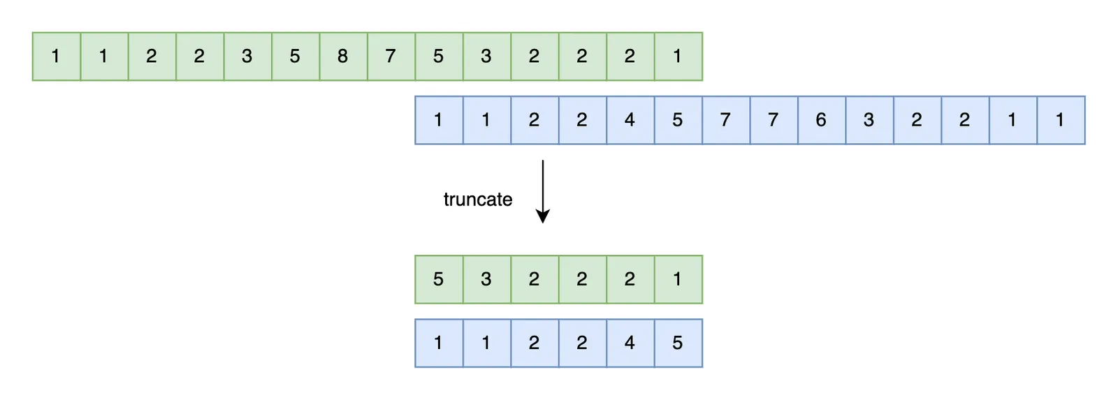
The previous statistics blog in this series shows how to use histograms as proxies for table distributions to estimate filter selectivity. We will also use histograms to estimate join outputs. But intersecting two histograms is more involved than truncating one.
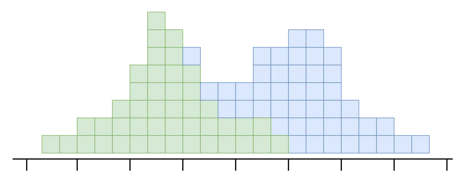
Consider intersecting the grasslands and forest histograms. Our first problem is that the buckets are non-overlapping. We need to truncate the tail of the forest histogram, whose values are all greater than the largest grasslands key.
Now that our histograms span the same key ranges, we need to align the two sets of bounds. One way to align buckets is to interpolate cut points using the other bucket’s boundaries. Lets suppose the last forest bucket is (80, 100) and the last grasslands bucket is (60, 100). We can cut the grasslands bucket in half to generate an alignment on (80) so that both histograms have a (80, 100) bucket. We cut all bounds with this strategy, distributing row and distinct counts between the two fractions.
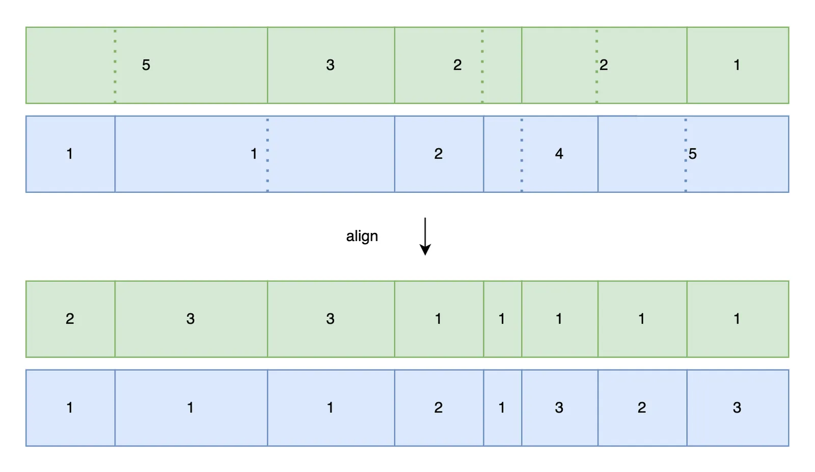
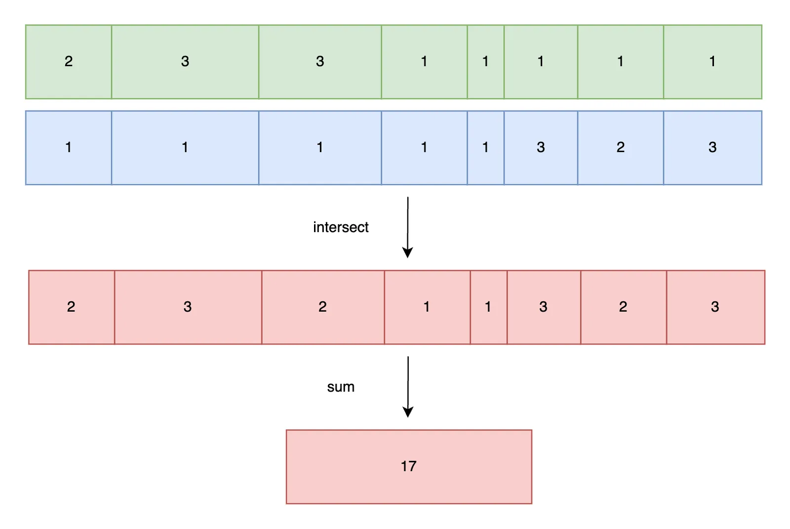
We now have what we’ve been waiting for! Two pairwise comparable histograms. If we estimate the number of join rows per bucket, the sum of all bucket-wise estimates approximates the join cardinality.
If we “multiply” two aligned buckets assuming the worst case Cartesian join
scenario, there will be mxn output rows. For example, two 10 row
buckets all with the same daily rainfall will generate 100 (year, year)
pairs. But this is only accurate when each bucket only contains one distinct
row. At the other extreme, if each bucket has no duplicate values
(distinct count = row count), the join can only return the minimum of
m and n. If grasslands has 10 unique keys in a bucket, and forest
has 100 unique keys, the result set can’t contain more than 10 unique
keys.
We average to even out the two extremes. We assume every key in the bucket with fewer rows will have a match in the larger set. But we also assume that distinct keys are distributed evenly; e.g. if a bucket has 100 rows and 10 unique keys, we assume each key has a frequency of 1/10, or equivalently, there are 10 copies of each key.
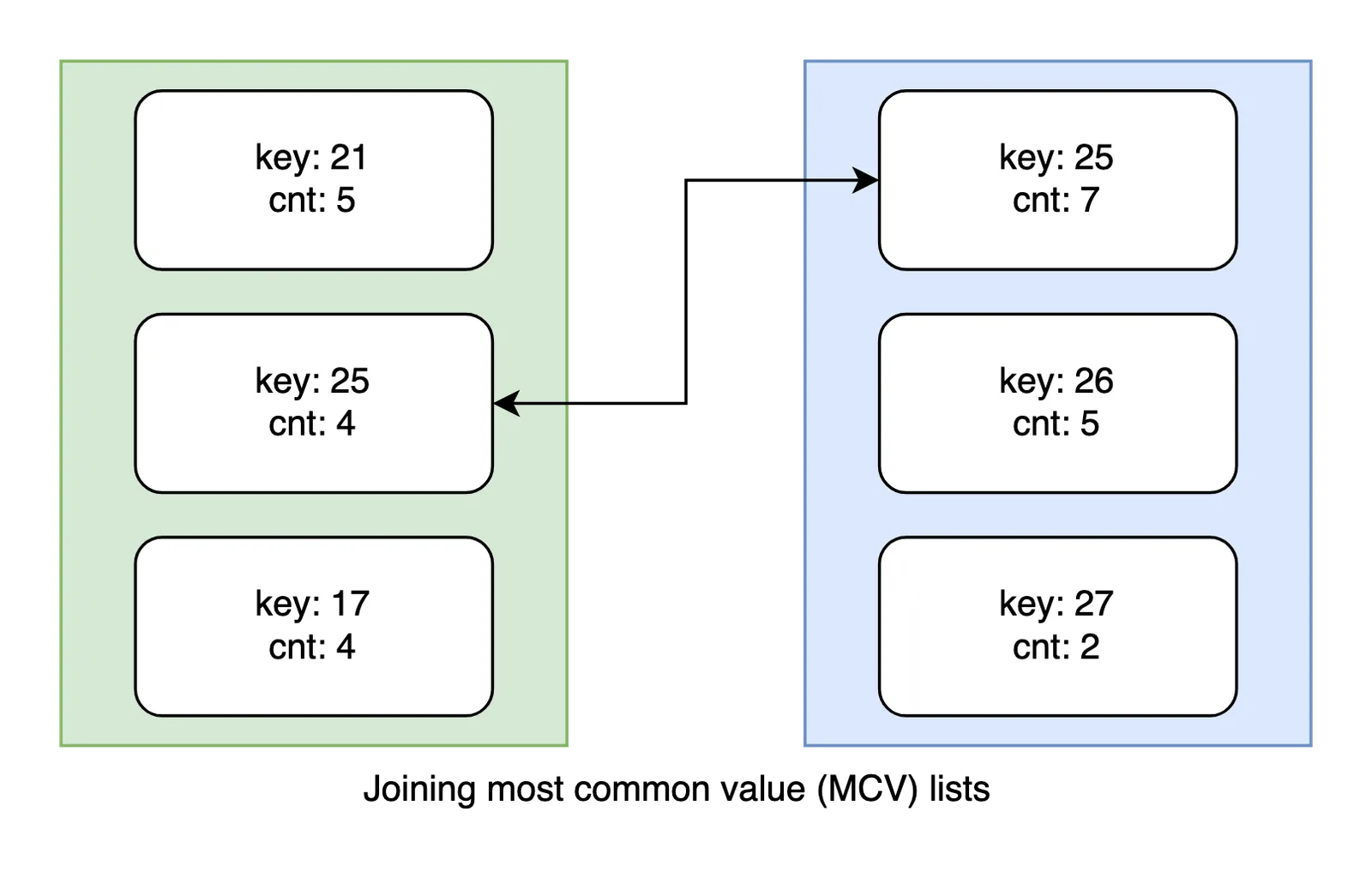
No real database is the average case with a perfectly uniform key distribution. Zipf’s Law is used to explain the phenomenon that datasets usually have a few keys that hog a disproportionate fraction of row space. We track these outliers “most common value” (MCV) sets and frequencies. MCVs are directly netted and joined separately from the otherwise uniformly estimated keys.
Below is a plot of the runtime pairwise baseline cardinalities compared to out histogram estimates. As with indexes, join estimates are fairly lossy. Fortunately, estimates only have to be accurate relative to each other to choose optimal plans.
| join | rows | estimate |
|---|---|---|
| DxG | 83895 | 7862 |
| GxF | 2171 | 2349 |
| FxD | 1905 | 495 |
We predict (accurately) that joining the forest and desert tables will create the smallest intermediate result. Because all paths converge after the last table is joined, plans beginning with DxG or GxF will be strictly more expensive. DxG is particularly expensive, for example, because it generates 80k intermediate rows compared to only 1900 for FxD. (DxG)xF then will join (80,000 x 1000) rows compared to (FxD)xG’s (1900)x(1000) rows.
Estimating join-filter queries and join-join queries is even more complicated, but the general process is the same. Estimates try to track upper-bound cardinalities. The accuracy granularities depend on how many histogram buckets we have. We use a combination of intra-bucket uniformity, with most common values tracked separately.
Future#
We will post a follow-up announcement soon with automatic refresh and lifecycle management for server statistics. Prolly trees’ structural sharing gives interesting options for how to update histogram buckets.
In the meantime, we will continue to test and improve the breadth and accuracy of estimates.
If you have any questions about Dolt, databases, or Golang performance reach out to us on Twitter, Discord, and GitHub!