
Dolt is the only version controlled relational database. Like if MySQL and Git had a baby, this baby also inherited the trauma of both parents. Today we will be talking about the SQL half.
Our users send us increasingly complicated queries in need of
performance optimizations. We want to formalize and hone how we address
these problems. This blog walks through how to debug slow queries. We
start by decomposing a query into its constituent parts. Then we
simplify the query to iterate more quickly. Finally we use
EXPLAIN queries, runtime profiles, and join hints to inspect and optimize.
Refer to the larger performance optimization reference for more details.
Simplifying Queries#
Decompose Query Into Parts#
Suppose a user reports this query as slow-running:
With cte1 as (
    Select category, elevation, count(*) as cnt
    from animals
    Group by category, elevation
), cte2 as (
    Select category, elevation, count(*) as cnt
    from plants p Group by category, elevation
), cte3 as (
    select *
    from cte1
    join cte2 on cte1.cnt = cte2.cnt
    where cte1.category = 7
)
select count(a.name)
from animals a
join plants p
     on a.category = p. category
join cte3 on
    a.elevation = cte3.elevation and
    a.category = cte3.category
where a.category = 7;
+---------------+
| count(a.name) |
+---------------+
| 10000000      |
+---------------+
________________________________________________________
Executed in   23.15 secs   fish           external
   usr time   23.51 secs  363.00 micros   23.51 secs
   sys time    0.21 secs  1202.00 micros    0.21 secs
The query has four distinct scopes, each of which we can examine individually:
cte1: aggregation onanimalscte2: aggregation onplantscte3: join betweencte1andcte2- Join between:
animalsxcte3xplants.
Let’s start by running the CTEs to estimate latency and row counts:
-- cte1
select count(*) from (
    select category, elevation, count(*) as cnt
    from animals group by category, elevation
) s;
+----------+
| count(*) |
+----------+
| 4003     |
+----------+
________________________________________________________
Executed in  257.79 millis    fish           external
   usr time  226.65 millis  114.00 micros  226.53 millis
   sys time   41.67 millis  572.00 micros   41.10 millis

-- cte2
select count(*) from (
    select category, elevation, count(*) as cnt
    from plants p group by category, elevation
) s;
+----------+
| count(*) |
+----------+
| 4003     |
+----------+
________________________________________________________
Executed in  394.93 millis    fish           external
   usr time  262.36 millis  119.00 micros  262.25 millis
   sys time   71.74 millis  620.00 micros   71.12 millis

-- cte3
with cte1 as (
  Select category, elevation, count(*) as cnt
  from animals
  Group by category, elevation
), cte2 as (
  select category, elevation, count(*) as cnt
  from plants p group by category, elevation
)
select count(*) from
    (
    select *
    from cte1
    join cte2 on cte1.cnt = cte2.cnt
    where cte1.elevation = 0 and
          cte2.elevation = 1
) s;
+----------+
| count(*) |
+----------+
| 400      |
+----------+
________________________________________________________
Executed in  224.48 millis    fish           external
   usr time  109.22 millis  140.00 micros  109.08 millis
   sys time   55.12 millis  660.00 micros   54.46 millis
(We wrap every query in this deep dive with a select count(*) from (...) s to avoid long output result sets and quickly summarize the
number of output rows for a scope.)
No CTE stands out as particularly expensive. We’ll look at the base tables next:
-- animals
select count(*) from animals;
+----------+
| count(*) |
+----------+
| 200003   |
+----------+
________________________________________________________
Executed in  433.95 millis    fish           external
   usr time  111.08 millis  121.00 micros  110.96 millis
   sys time   75.68 millis  612.00 micros   75.07 millis

-- plants
select count(*) from plants;
+----------+
| count(*) |
+----------+
| 200003   |
+----------+
________________________________________________________
Executed in  234.20 millis    fish           external
   usr time  117.26 millis  136.00 micros  117.12 millis
   sys time   58.89 millis  687.00 micros   58.21 millis
The plants and animals tables are a lot bigger than the CTEs.
We could test the [cte3 x plants] and [cte3 x animals] joins, but in
this case the [200_000 x 200_000] join looks more suspicious:
-- [plants x animals]
select count(*) from (
    select p.category, p.name, a.name
    from animals a join plants p
    on a.category = p. category
    where a.category = 7
) s;
+----------+
| count(*) |
+----------+
| 2500     |
+----------+
________________________________________________________
Executed in   18.81 secs   fish           external
   usr time   18.55 secs   85.23 millis   18.47 secs
   sys time    0.19 secs   24.21 millis    0.17 secs
We have a potential culprit! The cardinality (number of output rows) is not particularly high, but joining these two tables took almost 20 seconds.
Abbreviate Runtime#
When possible, we prefer debugging abbreviated versions of long-running queries. At the end of the day we’ll run the query dozens or hundreds of times while experimenting. Small changes in latency will save us time.
An ideal abbreviated query should take about a second. If we make the query too short, the overhead of printing results dominates the runtime (see profiles below for how to quantify overhead).
The first way to shorten a query is a LIMIT clause. This forces the
join to short-circuit after a specified number of rows are matched:
select count(*) from (
    select p.category, p.name, a.name
    from animals a join plants p
    on a.category = p. category
    where a.category = 7
    limit 10
) s;
+----------+
| count(*) |
+----------+
| 200      |
+----------+
________________________________________________________
Executed in    1.56 secs   fish           external
   usr time  1294.20 millis  137.00 micros  1294.06 millis
   sys time   75.01 millis  657.00 micros   74.35 millis
The limit reduces the cardinality (output row count) of the whole join, exiting after 200 matched rows. This strategy works when a query has a high cardinality and each row is an opportunity to exit early.
Joins that return few or no rows are more difficult because they expose no exit hooks. In that case, we need to reduce the cardinality of the join inputs (make join leafs return fewer rows).
First, we can LIMIT the cardinality of subscopes:
select count(*) from (
select p.category, p.name, a.name
from animals a join (select * from plants limit 10000) p
on a.category = p. category
where a.category = 7
) s;
+----------+
| count(*) |
+----------+
| 150      |
+----------+
________________________________________________________
Executed in    1.07 secs   fish           external
   usr time  1027.69 millis  141.00 micros  1027.55 millis
   sys time   54.34 millis  720.00 micros   53.62 millis
Unfortunately, the extra subquery makes plants unavailable for
LOOKUP_JOIN or MERGE_JOIN optimizations (more in later sections).
Optimizing a simplified query with a different execution plan is
harder to port back to the parent query.
Adding filters is the second way to abbreviate a table’s cardinality
(number of output rows). Below we add a filter to plants that will
makes the join [2500 x 200_000] rather than [200_000 x 200_000] (you
could also argue that the after is [2500 x 2500], depending on the
join strategy.)
select count(*) from (
    select p.category, p.name, a.name
    from animals a join plants p
    on a.category = p. category
    where a.category = 7 and
          p.category = 7
) s;
+----------+
| count(*) |
+----------+
| 2500     |
+----------+
________________________________________________________
Executed in    1.62 secs   fish           external
   usr time  895.93 millis  188.00 micros  895.75 millis
   sys time  131.42 millis  848.00 micros  130.58 millis
Tools For Debugging#
Explain Plan#
Tools for inspecting and correcting query execution are the bread and butter of performance debugging. Moreover, changes to a simplified query with a similar execution strategy as the original have the best chance of porting backwards.
The EXPLAIN query output peeks into a query’s execution plan,
describing how changes to a query string translate into an execution plan.
Returning to the original query:
+-------------------------------------------------------------------------------------------------------------+
| plan                                                                                                        |
+-------------------------------------------------------------------------------------------------------------+
| GroupBy                                                                                                     |
|  ├─ SelectedExprs(COUNT(a.name))                                                                            |
|  ├─ Grouping()                                                                                              |
|  └─ HashJoin                                                                                                |
|      ├─ ((a.elevation = cte3.elevation) AND (a.category = cte3.category))                                   |
|      ├─ SubqueryAlias                                                                                       |
|      │   ├─ name: cte3                                                                                      |
|      │   ├─ outerVisibility: false                                                                          |
|      │   ├─ cacheable: true                                                                                 |
|      │   └─ Project                                                                                         |
|      │       ├─ columns: [cte1.category, cte1.elevation, cte1.cnt, cte2.category, cte2.elevation, cte2.cnt] |
|      │       └─ HashJoin                                                                                    |
|      │           ├─ (cte1.cnt = cte2.cnt)                                                                   |
|      │           ├─ SubqueryAlias                                                                           |
|      │           │   ├─ name: cte2                                                                          |
|      │           │   ├─ outerVisibility: false                                                              |
|      │           │   ├─ cacheable: true                                                                     |
|      │           │   └─ Project                                                                             |
|      │           │       ├─ columns: [p.category, p.elevation, COUNT(1) as cnt]                             |
|      │           │       └─ GroupBy                                                                         |
|      │           │           ├─ SelectedExprs(p.category, p.elevation, COUNT(1))                            |
|      │           │           ├─ Grouping(p.category, p.elevation)                                           |
|      │           │           └─ TableAlias(p)                                                               |
|      │           │               └─ Table                                                                   |
|      │           │                   ├─ name: plants                                                        |
|      │           │                   └─ columns: [category elevation]                                       |
|      │           └─ HashLookup                                                                              |
|      │               ├─ outer: (cte2.cnt)                                                                   |
|      │               ├─ inner: (cte1.cnt)                                                                   |
|      │               └─ CachedResults                                                                       |
|      │                   └─ SubqueryAlias                                                                   |
|      │                       ├─ name: cte1                                                                  |
|      │                       ├─ outerVisibility: false                                                      |
|      │                       ├─ cacheable: true                                                             |
|      │                       └─ Project                                                                     |
|      │                           ├─ columns: [animals.category, animals.elevation, COUNT(1) as cnt]         |
|      │                           └─ GroupBy                                                                 |
|      │                               ├─ SelectedExprs(animals.category, animals.elevation, COUNT(1))        |
|      │                               ├─ Grouping(animals.category, animals.elevation)                       |
|      │                               └─ IndexedTableAccess(animals)                                         |
|      │                                   ├─ index: [animals.category]                                       |
|      │                                   ├─ filters: [{[7, 7]}]                                             |
|      │                                   └─ columns: [category elevation]                                   |
|      └─ HashLookup                                                                                          |
|          ├─ outer: (cte3.elevation, cte3.category)                                                          |
|          ├─ inner: (a.elevation, a.category)                                                                |
|          └─ CachedResults                                                                                   |
|              └─ LookupJoin                                                                                  |
|                  ├─ (a.category = p.category)                                                               |
|                  ├─ TableAlias(p)                                                                           |
|                  │   └─ Table                                                                               |
|                  │       ├─ name: plants                                                                    |
|                  │       └─ columns: [category]                                                             |
|                  └─ Filter                                                                                  |
|                      ├─ (a.category = 7)                                                                    |
|                      └─ TableAlias(a)                                                                       |
|                          └─ IndexedTableAccess(animals)                                                     |
|                              ├─ index: [animals.category]                                                   |
|                              └─ columns: [name category elevation]                                          |
+-------------------------------------------------------------------------------------------------------------+
There is a lot of output, but we can break it down step by step. Refer to the diagram below for a visualization (the join tree is tagged blue).
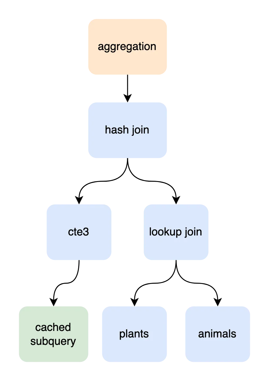
The entry level scope is an aggregation projecting COUNT(a.name). The main
input into that aggregation is a three-way join between cte3, plants, and
animals.
The [plants x animals] LOOKUP_JOIN constructs a (category) key for
every plant row to index into animals.category.
The cte3 x [plants x animals] HASH_JOIN places each row returned by
[plants x animals] into an in-memory hash map keyed by animals.category.
The first row from cte3 scans all rows from the join-right, but every other
row from cte3 probes the hash map for matches.
cte3 clutters the EXPLAIN output, but the information helps reaffirm
the safety of our simplified query. We have identified that cte3
executes quickly. And we can see here that cte3 is cached and will
only execute once, limiting its impact on the larger join.
Now let’s look at the plan for the simplified query ([plants x animals]):
explain
select p.category, p.name, a.name
from animals a join plants p
on a.category = p. category
where a.category = 7

+-----------------------------------------------+
| plan                                          |
+-----------------------------------------------+
| Project                                       |
|  ├─ columns: [p.category, p.name, a.name]     |
|  └─ LookupJoin                                |
|      ├─ (a.category = p.category)             |
|      ├─ TableAlias(p)                         |
|      │   └─ Table                             |
|      │       ├─ name: plants                  |
|      │       └─ columns: [name category]      |
|      └─ Filter                                |
|          ├─ (a.category = 7)                  |
|          └─ TableAlias(a)                     |
|              └─ IndexedTableAccess(animals)   |
|                  ├─ index: [animals.category] |
|                  └─ columns: [name category]  |
+-----------------------------------------------+
This is much easier to read! If we look closely, we can see how the
simplified join strategy maps to the original
plan: LOOKUP_JOIN(plants, animals, (a.category=p.category)).
CPU Profiles#
Before we start debugging, we have one last tool for understanding slow queries: profiling.
A query string is the basic request of what to execute. The query plan is how the engine will run the query. And a profile tells us what the CPU was doing while executing the query.
Showing will be easier than explaining, so let’s run a profile with our simplified query:
dolt --prof cpu sql -q "
  select /*+ LOOKUP_JOIN(a,p) */ p.category, p.name, a.name
  from animals a join plants p
  on a.category = p. category
  where a.category = 7
    limit 200
"
cpu profiling enabled.
2023/03/22 10:52:32 profile: cpu profiling enabled, /var/folders/h_/n5qdj2tj3n741n128t7v2d7h0000gn/T/profile3980486175/cpu.pprof
...
2023/03/22 10:52:33 profile: cpu profiling disabled, /var/folders/h_/n5qdj2tj3n741n128t7v2d7h0000gn/T/profile3980486175/cpu.pprof
Profiles include an enormous amount of detail and track the number of milliseconds spent running every line of source code. I prefer starting with the top-down flamegraph to orient myself to the larger picture:
> go tool pprof -http :8080 /var/folders/h_/n5qdj2tj3n741n128t7v2d7h0000gn/T/profile3980486175/cpu.pprof
Serving web UI on http://localhost:8080
Opening http://localhost:8080/flamegraph…
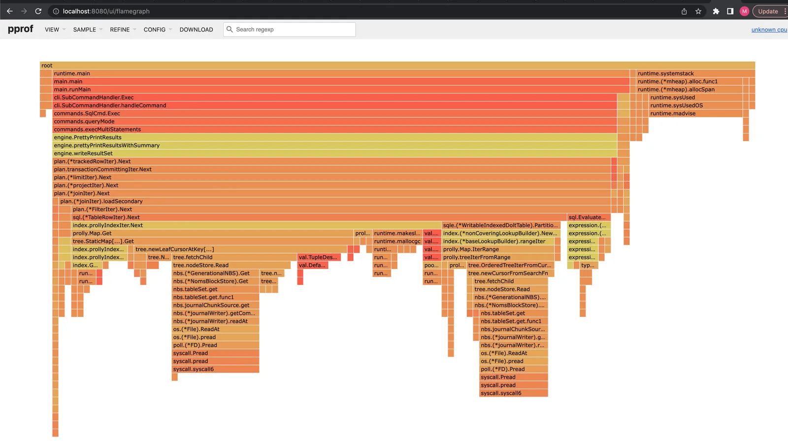
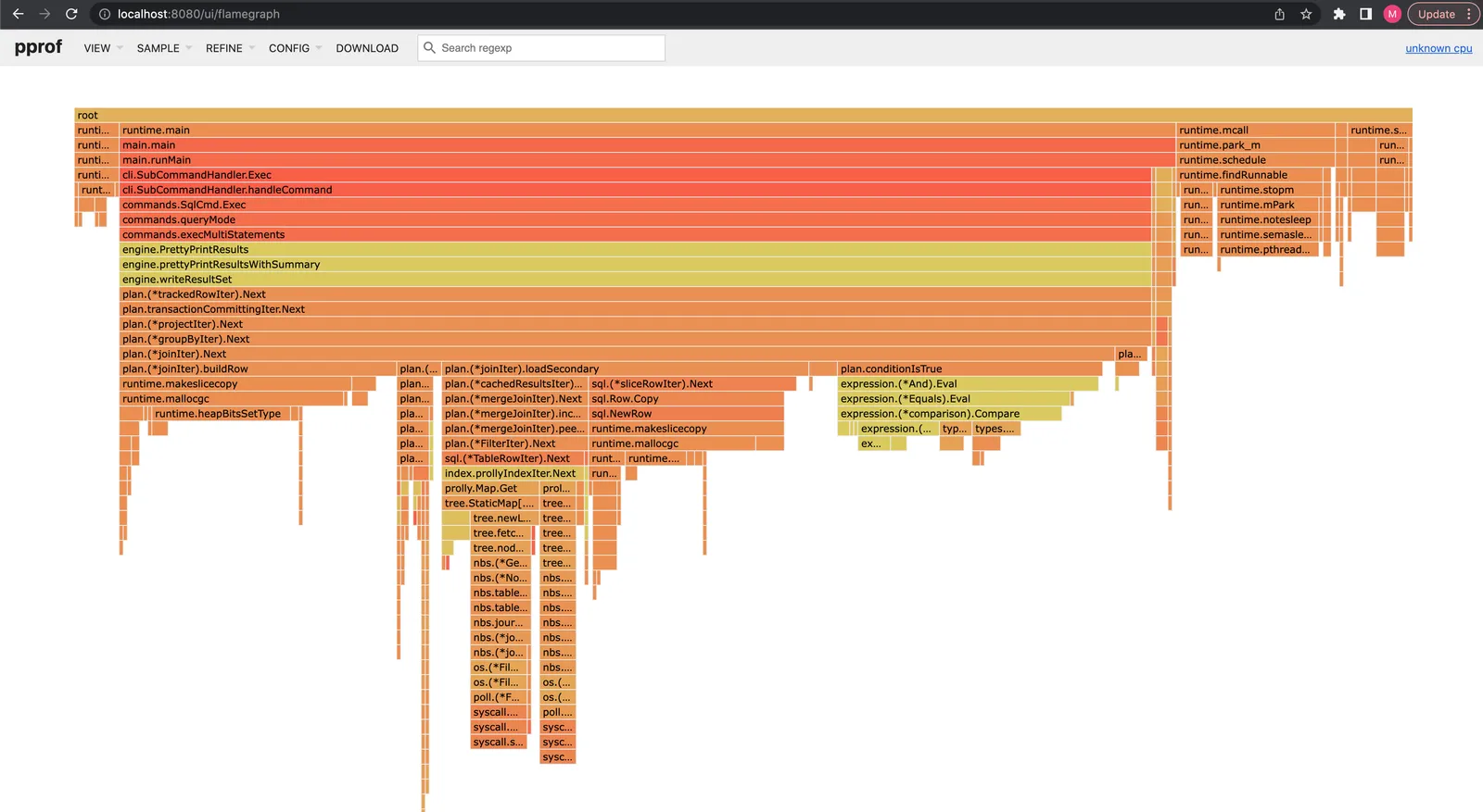
The flamegraph is an aggregated call stack. Vertical bars are nested function calls. The width of a specific bar indicates the amount of time the active call stack included a function. The standalone amount of time spent executing a single function is the width of its bar minus the width of its subroutines.
We spend 80% of the total query time in loadSecondary
(reading animals). 5% is spent executing filter logic, and 75% is
spent getting rows from disk into the filter operator. As a comparison,
we spend less than 1% of the runtime reading rows from plants (the
sliver to the left of loadSecondary under joinIter.Next).
Another clue is the non-covering lookup. The profile shows
that we do two expensive disk-accesses within each loadSecondary. One
finds a matching index entry, and the second probes the primary key to
fill out missing fields.
The last observation is that we spend 15% of runtime performing garbage collection. This is a lot of GC, but not as practical to fix as a user.
Debug A Query#
We have a simplified query and background on how to use EXPLAINs and
profiles to gather data. The only thing left to do is experiment with
perf improvements from the performance
reference.
Covering index#
The profile suggested a covering index would improve latency. Let’s add an index that solves that problem:
alter table animals add index (category, name);The new index preserves the lookup on category, but includes name
in the index to avoid referencing the primary key:
+------------------------------------------------------------------------+
| plan                                                                   |
+------------------------------------------------------------------------+
| GroupBy                                                                |
|  ├─ SelectedExprs(COUNT(1))                                            |
|  ├─ Grouping()                                                         |
|  └─ SubqueryAlias                                                      |
|      ├─ name: s                                                        |
|      ├─ outerVisibility: false                                         |
|      ├─ cacheable: true                                                |
|      └─ Limit(200)                                                     |
|          └─ Project                                                    |
|              ├─ columns: [p.category, p.name, a.name]                  |
|              └─ LookupJoin                                             |
|                  ├─ (a.category = p.category)                          |
|                  ├─ TableAlias(p)                                      |
|                  │   └─ Table                                          |
|                  │       ├─ name: plants                               |
|                  │       └─ columns: [name category]                   |
|                  └─ Filter                                             |
|                      ├─ (a.category = 7)                               |
|                      └─ TableAlias(a)                                  |
|                          └─ IndexedTableAccess(animals)                |
|                              ├─ index: [animals.category,animals.name] |
|                              └─ columns: [name category]               |
+------------------------------------------------------------------------+
The profile shows that we now spend ~70% of runtime in loadSecondary now,
an improvement from ~80%:
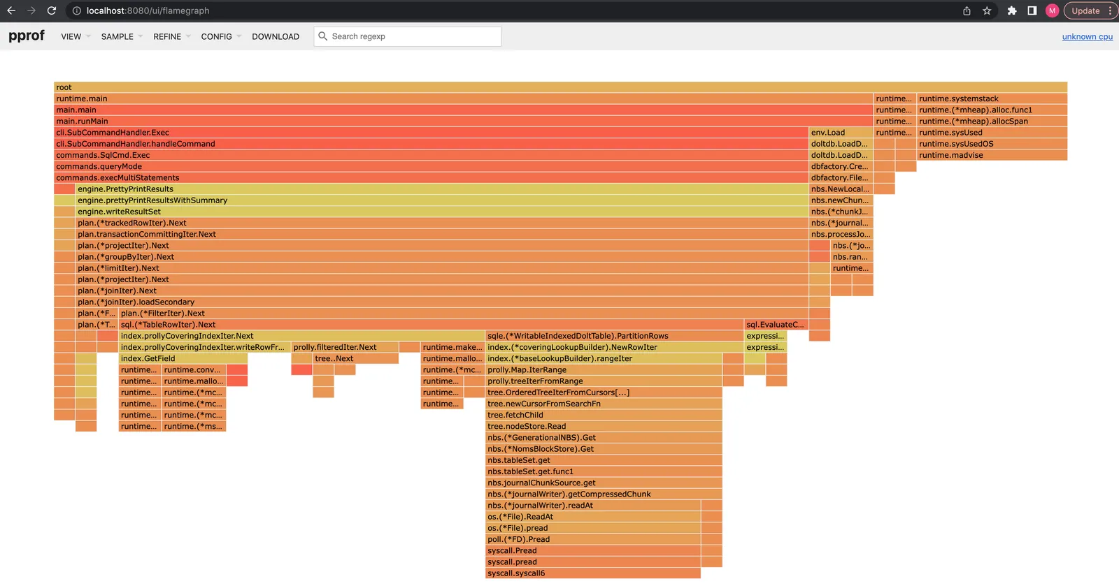
The latency difference is even more dramatic: 800ms compared to 1.6 seconds before:
...
+----------+
| count(*) |
+----------+
| 200      |
+----------+
________________________________________________________
Executed in  788.94 millis    fish           external
   usr time  540.78 millis  137.00 micros  540.64 millis
   sys time   64.95 millis  741.00 micros   64.21 millis
Join Hints#
Every database is subject to performance pitfalls. In general there are O(n!) possible plans for an n-table join. Estimating the cost of executing each relies on statistical guesses that are expensive to maintain, and can still guess wrong when perfectly up-to-date.
Query hints are a common tool to take manual control over the engine to force execution paths when the optimizer picks a slow plan. We will compare the latency of every two-table join execution plan for our simple query using hints.
Dolt’s join hints are indicated in comment brackets immediately
after a SELECT clause and before the projected columns, like this:
SELECT /*+ JOIN_HINT1 JOIN_HINT2 */ .... The optimizer tries to
apply all hints, but will fallback to a default plan if all hints are
not satisfied.
One hint that will be useful is JOIN_ORDER, which indicates a desired
join tree table order:
select /*+ JOIN_ORDER(a,p) */ p.category, p.name, a.name
from animals a join plants p
on a.category = p. category
where a.category = 7
limit 200
The join operator hints will also come in handy: INNER_JOIN, LOOKUP_JOIN, HASH_JOIN,
MERGE_JOIN:
select /*+ MERGE_JOIN(a,p) */ p.category, p.name, a.name
from animals a join plants p
on a.category = p. category
where a.category = 7
limit 200
Here is a latency plot of our simplified query with every combination of join orders and operators:
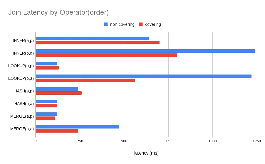
One takeaway is the JOIN_ORDER(a,p) is generally faster than
JOIN_ORDER(p,a). We rationalize this by observing that the filters on
animals reduces its cardinality to 2500 rows, but plants returns a
full 200,000 rows. A lookup join from animals -> plants performs
2500 lookups into plants. On the other hand, a lookup join from plants
-> animals performs 200,000 lookups.
HASH_JOIN and MERGE_JOINs also perform better than LOOKUP_JOINs on average. HASH_JOIN performs well for small tables that fit in memory, but are prohibitively expensive for large tables. MERGE_JOINs require indexes on both table relations, and can only be applied rarely. But when available MERGE_JOIN out-performs other join strategies. This is particularly true for LOOKUP_JOIN, whose random access incurs a scaling penalty on large tables.
Testing On Original Query#
We squeezed the simplified query from 1.5 seconds down to 110 milliseconds, but we need to make sure our improvements generalize to the original.
We add /*+ JOIN_ORDER(cte3,a,p) HASH_JOIN(cte3,a) MERGE_JOIN(a,p) */
as a hint below to include cte3 in our desired plan:
explain
With cte1 as (
Select category, elevation, count(*) as cnt
from animals
Group by category, elevation
), cte2 as (
Select category, elevation, count(*) as cnt
from plants p Group by category, elevation
), cte3 as (
select *
from cte1
join cte2 on cte1.cnt = cte2.cnt
where cte1.category = 7
)
select /*+ JOIN_ORDER(cte3,a,p) HASH_JOIN(cte3,a) MERGE_JOIN(a,p) */ count(a.name)
from animals a
join plants p
on a.category = p. category
join cte3 on
a.elevation = cte3.elevation and
a.category = cte3.category
where a.category = 7;
+-------------------------------------------------------------------------------------------------------------+
| plan |
+-------------------------------------------------------------------------------------------------------------+
| GroupBy |
| ├─ SelectedExprs(COUNT(a.name)) |
| ├─ Grouping() |
| └─ HashJoin |
| ├─ ((a.elevation = cte3.elevation) AND (a.category = cte3.category)) |
| ├─ SubqueryAlias |
| │ ├─ name: cte3 |
| │ ├─ outerVisibility: false |
| │ ├─ cacheable: true |
| │ └─ Project |
| │ ├─ columns: [cte1.category, cte1.elevation, cte1.cnt, cte2.category, cte2.elevation, cte2.cnt] |
| │ └─ HashJoin |
| │ ├─ (cte1.cnt = cte2.cnt) |
| │ ├─ SubqueryAlias |
| │ │ ├─ name: cte2 |
| │ │ ├─ outerVisibility: false |
| │ │ ├─ cacheable: true |
| │ │ └─ Project |
| │ │ ├─ columns: [p.category, p.elevation, COUNT(1) as cnt] |
| │ │ └─ GroupBy |
| │ │ ├─ SelectedExprs(p.category, p.elevation, COUNT(1)) |
| │ │ ├─ Grouping(p.category, p.elevation) |
| │ │ └─ TableAlias(p) |
| │ │ └─ Table |
| │ │ ├─ name: plants |
| │ │ └─ columns: [category elevation] |
| │ └─ HashLookup |
| │ ├─ outer: (cte2.cnt) |
| │ ├─ inner: (cte1.cnt) |
| │ └─ CachedResults |
| │ └─ SubqueryAlias |
| │ ├─ name: cte1 |
| │ ├─ outerVisibility: false |
| │ ├─ cacheable: true |
| │ └─ Project |
| │ ├─ columns: [animals.category, animals.elevation, COUNT(1) as cnt] |
| │ └─ GroupBy |
| │ ├─ SelectedExprs(animals.category, animals.elevation, COUNT(1)) |
| │ ├─ Grouping(animals.category, animals.elevation) |
| │ └─ IndexedTableAccess(animals) |
| │ ├─ index: [animals.category] |
| │ ├─ filters: [{[7, 7]}] |
| │ └─ columns: [category elevation] |
| └─ HashLookup |
| ├─ outer: (cte3.elevation, cte3.category) |
| ├─ inner: (a.elevation, a.category) |
| └─ CachedResults |
| └─ MergeJoin |
| ├─ cmp: (a.category = p.category) |
| ├─ Filter |
| │ ├─ (a.category = 7) |
| │ └─ TableAlias(a) |
| │ └─ IndexedTableAccess(animals) |
| │ ├─ index: [animals.category] |
| │ ├─ filters: [{[NULL, ∞)}] |
| │ └─ columns: [name category elevation] |
| └─ TableAlias(p) |
| └─ IndexedTableAccess(plants) |
| ├─ index: [plants.category] |
| ├─ filters: [{[NULL, ∞)}] |
| └─ columns: [category] |
+-------------------------------------------------------------------------------------------------------------+The plan includes a [animals x plants] merge join and cte3 x [animals x plants]
hash join.
The latency improve from ~20 seconds down to ~3 seconds when running the hinted plan:
+---------------+
| count(a.name) |
+---------------+
| 10000000      |
+---------------+
________________________________________________________
Executed in    3.11 secs   fish           external
   usr time    3.78 secs   92.87 millis    3.69 secs
   sys time    0.20 secs  108.25 millis    0.10 secs
And finally, here is the performance profile of the hinted query. We spend
as much time building the row (joinIter.buildRow 20%) and evaluating the
join condition (conditionIsTrue 20%) as we do reading data from disk
(loadPrimary 3%, loadSecondary 27%).
Summary#
We walked through how to debug a slow join. First we simplified the query
and used a LIMIT to return more quickly. Then
we discussed how EXPLAIN query and profile are valuable tools for inspecting
performance. We tested replacing a non-convering index lookup with a covering
index. And finally,
we used join hints to compare the performance of every two-table join strategy.
Debugging slow queries is increasingly difficult for big joins on big tables. But the strategy remains the same: break a query into smaller manageable components. Use EXPLAIN and CPU profiles to identify and debug the thorniest components. Use indexes to limit the number of disk accesses, push low cardinality tables as low in join trees.
When we find a slow join, we always prefer adding internal optimizations > adding query hints > adding table indexes > rearranging queries, in that order. But we also need to find workarounds to ways for customers to investigate themselves. Hopefully this is is a useful how-to for those of you interested in trying yourselves.
Refer to the optimization reference for more details on common optimization patterns.
If you have any questions about Dolt, databases, or Golang performance reach out to us on Twitter, Discord, and GitHub!