Dolt Vs MySQL Vs Postgres

June 23, 2023

18 min read

Dolt was originally designed as a standalone CLI tool for supporting distributed asynchronous data sharing with the same primitives as Git. But we are now a database company. We still support data sharing with Git semantics but increasingly in a client-server model. Two blogs the the last week color this focus; rewiring CLI commands as SQL queries, and the latest status on our hosted service, our managed support for customers with long-running database servers.

The increasing number of customers using Dolt as a database service (including us) adds scrutiny to the engine.

Database engines 1) interpret strings as well formed queries, 2) convert the query into optimal plans, and 3) execute planned statements. The order of interpret, plan, execute is chronologically how database engines work, but also the order transactional databases improve over time. So far we have spent most of our time doing (1), covering the MySQL syntax dialect and building a testing suite of execution correctness. We dip into (2) for key areas like join planning. But for the most part Dolt has yet to take advantage of modern statistical costing (2) and execution (3).

So it was a surprise when a customer reported a slow query where Dolt already beat MySQL. This blog does a Dolt versus MySQL comparison to see how far we have come. We also add a Dolt vs Postgres comparison to splash a bit of cold water on our victory lap and see where improving costing and execution will take us.

Slow Aggregation Query

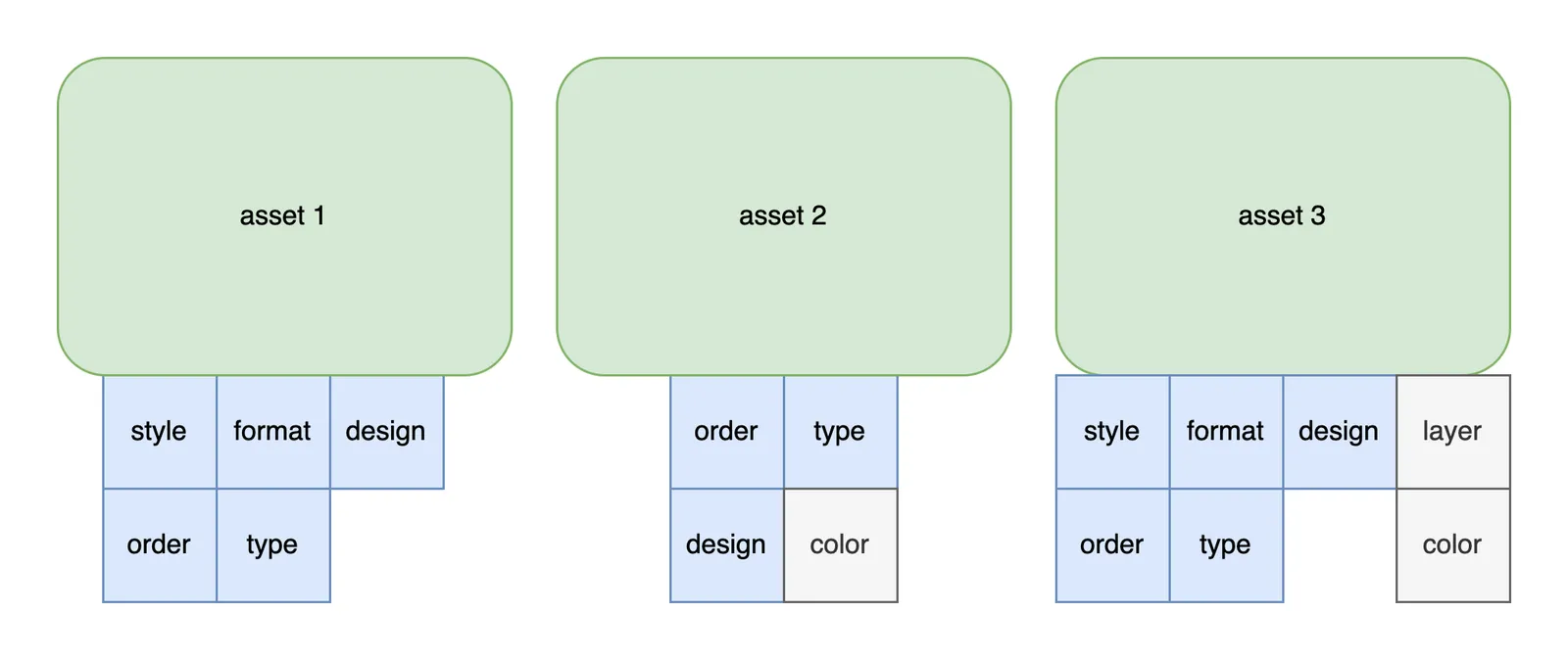
The example database is a digital warehouse tracking assets and asset attributes. The cartoon diagram below is simplistic, but basically we segregate core assets into one table and their attributes in a second. We would join the two tables on assetId to gather all of the info for a single asset.

The target query only reads the attributes table, outputting a set of assets that match a current set of criteria:

select
  `assetId` from `assets_metadata`
where
  `name` = 'Design' and
  `value` = 'VIBE' and
  `orgId` = '1'
  or
  `name` = 'Style' and
  `value` = 'Blank' and
  `orgId` = '1'
  or
  `name` = 'Order' and
  `value` = '1' and  
  `orgId` = '1'
  or
  `name` = 'Type' and
  `value` = 'Layer' and
  `orgId` = '1'
  or
  `name` = 'Format' and
  `value` = 'Vector' and
  `orgId` = '1'
group by `assetId`
having count(assetId) = 5;

We want assets with the list of associated attributes: design, style, order, type, format. The assets may have other attributes, but they need to have at least the 5 requested. In the diagram, the first asset's attributes intersect our search set, the second asset is missing attributes, and the third asset has more attributes than the search set. The GROUP_BY and HAVING clauses select asset 1 and 3 and remove 2.

Dolt vs MySQL

Benchmarking in MySQL:

+--------------------------------------+
| assetId                              |
+--------------------------------------+
| b7ceddac-7461-400a-a2d3-696c9d34e138 |
| e4bd82cc-27f4-4165-b7d6-7feaa786ec1f |
+--------------------------------------+
2 rows in set (0.66 sec)

And in Dolt:

+--------------------------------------+
| assetId                              |
+--------------------------------------+
| b7ceddac-7461-400a-a2d3-696c9d34e138 |
| e4bd82cc-27f4-4165-b7d6-7feaa786ec1f |
+--------------------------------------+
2 rows in set (0.56 sec)

660ms vs 560ms isn't a huge difference, but we'll take it!

The Dolt and MySQL plans are pretty similar. Both use an index to fuzzy range scan a subset of the table, filter rows for exact matches, aggregate on assetId, and return matches with 5 attributes.

Here is the MySQL plan:

-> Filter: (count(assets_metadata.assetId) = 5)  (cost=2104.21 rows=4135) (actual time=762.597..1021.153 rows=2 loops=1)
    -> Group aggregate: count(assets_metadata.assetId)  (cost=2104.21 rows=4135) (actual time=0.164..1016.769 rows=22340 loops=1)
        -> Filter: (((assets_metadata.orgId = '8f0e4d53-41c5-4d8d-9765-e0b1e625dee1') and (assets_metadata.`value` = 'VIBE') and (assets_metadata.`name` = 'Design')) or ((assets_metadata.orgId = '8f0e4d53-41c5-4d8d-9765-e0b1e625dee1') and (assets_metadata.`value` = 'JS96W') and (assets_metadata.`name` = 'Style')) or ((assets_metadata.orgId = '8f0e4d53-41c5-4d8d-9765-e0b1e625dee1') and (assets_metadata.`value` = '1') and (assets_metadata.`name` = 'Order')) or ((assets_metadata.orgId = '8f0e4d53-41c5-4d8d-9765-e0b1e625dee1') and (assets_metadata.`value` = 'Layer') and (assets_metadata.`name` = 'Type')) or ((assets_metadata.orgId = '8f0e4d53-41c5-4d8d-9765-e0b1e625dee1') and (assets_metadata.`value` = 'Vector') and (assets_metadata.`name` = 'Format')))  (cost=1690.73 rows=4135) (actual time=0.118..992.149 rows=43688 loops=1)
            -> Index lookup on assets_metadata using assets_metadata_orgid_assetid_index (orgId='8f0e4d53-41c5-4d8d-9765-e0b1e625dee1'), with index condition: ((assets_metadata.orgId = '8f0e4d53-41c5-4d8d-9765-e0b1e625dee1') or (assets_metadata.orgId = '8f0e4d53-41c5-4d8d-9765-e0b1e625dee1') or (assets_metadata.orgId = '8f0e4d53-41c5-4d8d-9765-e0b1e625dee1') or (assets_metadata.orgId = '8f0e4d53-41c5-4d8d-9765-e0b1e625dee1') or (assets_metadata.orgId = '8f0e4d53-41c5-4d8d-9765-e0b1e625dee1'))  (cost=1690.73 rows=84367) (actual time=0.110..768.183 rows=170383 loops=1)

And here is the Dolt plan:

Project
 ├─ columns: [assets_metadata.assetId]
 └─ Having((COUNT(assets_metadata.assetId) = 5))
     └─ GroupBy
         ├─ SelectedExprs(assets_metadata.assetId, COUNT(assets_metadata.assetId))
         ├─ Grouping(assets_metadata.assetId)
         └─ Filter
             ├─ (((((((assets_metadata.name = 'Design') AND (assets_metadata.value = 'VIBE')) AND (assets_metadata.orgId = '8f0e4d53-41c5-4d8d-9765-e0b1e625dee1')) OR (((assets_metadata.name = 'Style') AND (assets_metadata.value = 'JS96W')) AND (assets_metadata.orgId = '8f0e4d53-41c5-4d8d-9765-e0b1e625dee1'))) OR (((assets_metadata.name = 'Order') AND (assets_metadata.value = '1')) AND (assets_metadata.orgId = '8f0e4d53-41c5-4d8d-9765-e0b1e625dee1'))) OR (((assets_metadata.name = 'Type') AND (assets_metadata.value = 'Layer')) AND (assets_metadata.orgId = '8f0e4d53-41c5-4d8d-9765-e0b1e625dee1'))) OR (((assets_metadata.name = 'Format') AND (assets_metadata.value = 'Vector')) AND (assets_metadata.orgId = '8f0e4d53-41c5-4d8d-9765-e0b1e625dee1')))
             └─ IndexedTableAccess(assets_metadata)
                 ├─ index: [assets_metadata.orgId,assets_metadata.name,assets_metadata.value]
                 └─ filters: [{[8f0e4d53-41c5-4d8d-9765-e0b1e625dee1, 8f0e4d53-41c5-4d8d-9765-e0b1e625dee1], [Design, Design], [VIBE, VIBE]}, {[8f0e4d53-41c5-4d8d-9765-e0b1e625dee1, 8f0e4d53-41c5-4d8d-9765-e0b1e625dee1], [Format, Format], [Vector, Vector]}, {[8f0e4d53-41c5-4d8d-9765-e0b1e625dee1, 8f0e4d53-41c5-4d8d-9765-e0b1e625dee1], [Order, Order], [1, 1]}, {[8f0e4d53-41c5-4d8d-9765-e0b1e625dee1, 8f0e4d53-41c5-4d8d-9765-e0b1e625dee1], [Style, Style], [JS96W, JS96W]}, {[8f0e4d53-41c5-4d8d-9765-e0b1e625dee1, 8f0e4d53-41c5-4d8d-9765-e0b1e625dee1], [Type, Type], [Layer, Layer]}]

One difference is that MySQL uses a non-unique (orgId) index prefix for the innermost scan, while Dolt uses the key (orgId,name,value). MySQL perhaps does this because the index choice is unique, although the prefix is not. Dolt's more selective index reads fewer rows and returns sooner. Another oddity is that MySQL performs redundant and expensive assets_metadata.orgId = '8f0e4d53-41c5-4d8d-9765-e0b1e625dee1' filters.

Dolt vs Postgres

We usually compare ourselves to MySQL for historical reasons described here. But widening our base of comparison to include Postgres is informative. And we are already tying a closer relationship by exposing more Postgres-Dolt features, like a Postgres foreign data wrapper, and maybe a Postgres wire-compatible dialect for Dolt sql-server.

Here is the aggregation run in Postgres:

postgres=# select assetId from assets_metadata where   (name = 'Design' and value = 'VIBE' and   orgId = '8f0e4d53-41c5-4d8d-9765-e0b1e625dee1')    or   (name = 'Style' and value = 'JS96W' and   orgId = '8f0e4d53-41c5-4d8d-9765-e0b1e625dee1')   or (name = 'Order' and value = '1' and   orgId = '8f0e4d53-41c5-4d8d-9765-e0b1e625dee1')   or (name = 'Type' and value = 'Layer' and   orgId = '8f0e4d53-41c5-4d8d-9765-e0b1e625dee1')   or (name = 'Format' and value = 'Vector' and   orgId = '8f0e4d53-41c5-4d8d-9765-e0b1e625dee1') group by assetId having count(assetId) = 5;
               assetid
--------------------------------------
 b7ceddac-7461-400a-a2d3-696c9d34e138
 e4bd82cc-27f4-4165-b7d6-7feaa786ec1f
(2 rows)

Time: 62.931 ms

Postgres's aggregation has two main differences. First, they parallelize the index scan on the disjoint filter. Second, their range scan is not fuzzy and they eliminate the in-memory filter.

 Finalize HashAggregate  (cost=7636.38..7714.80 rows=31 width=37)
   Group Key: assetid
   Filter: (count(assetid) = 5)
   ->  Gather  (cost=7001.67..7607.52 rows=5770 width=45)
         Workers Planned: 2
         ->  Partial HashAggregate  (cost=6001.67..6030.52 rows=2885 width=45)
               Group Key: assetid
               ->  Parallel Seq Scan on assets_metadata  (cost=0.00..5987.25 rows=2885 width=37)
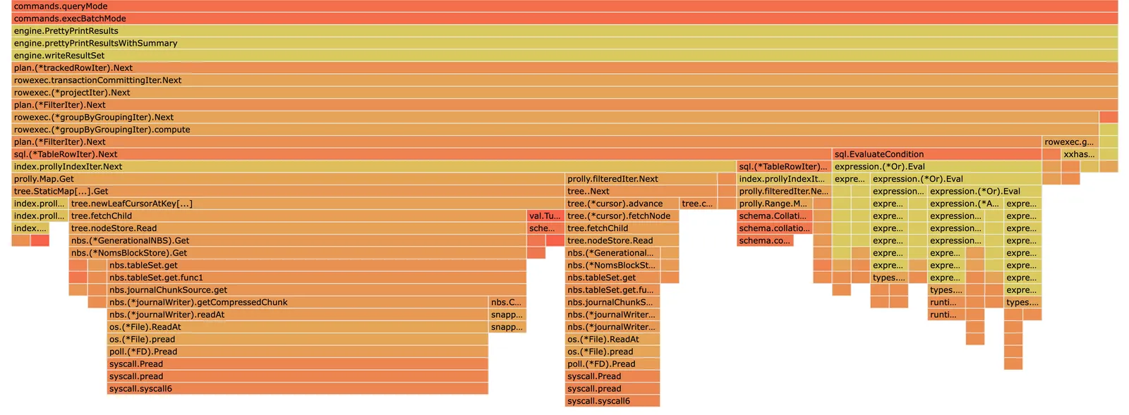
                     Filter: ((orgid = '8f0e4d53-41c5-4d8d-9765-e0b1e625dee1'::bpchar) AND ((((name)::text = 'Design'::text) AND ((value)::text = 'VIBE'::text)) OR (((name)::text = 'Style'::text) AND ((value)::text = 'JS96W'::text)) OR (((name)::text = 'Order'::text) AND ((value)::text = '1'::text)) OR (((name)::text = 'Type'::text) AND ((value)::text = 'Layer'::text)) OR (((name)::text = 'Format'::text) AND ((value)::text = 'Vector'::text))))

Looking at Dolt's performance profile, half of the 560ms Dolt latency is spent performing a filter. The 200ms we spend reading data off disk is a bit opaque without more research, but a hypothetical parallelization between two workers might bring us within earshot of Postgres at 100ms. Compression can also have a dramatic impact on queries rate limited by reading data off disk. A lot of orange to squeeze, but nothing out of our reach.

Rewriting The Aggregation As A Join

The original query scans the table, aggregates attributes by id, and counts the number for each asset. We pointed our customer towards using a join instead. A 5-way join with a lookup for each attribute selects the same set of assets:

select design.assetId
from assets_metadata design
join assets_metadata style
  on design.assetId = style.assetId
join assets_metadata `order`
  on design.assetId = `order`.assetId
join assets_metadata type
  on design.assetId = type.assetId
join assets_metadata `format`
  on design.assetId = `format`.assetId
where
  (design.`value` = 'VIBE' ) and
  (style.`value` = 'JS96W') and
  (`order`.`value` = '1') and
  (type.`value` = 'Layer') and
  (`format`.`value` = 'Vector') and
  (design.`name` = 'Design' ) and
  (style.`name` = 'Style') and
  (`order`.`name` = 'Order') and
  (type.`name` = 'Type') and
  (`format`.`name` = 'Format') and
  (design.`orgId` = '8f0e4d53-41c5-4d8d-9765-e0b1e625dee1') and
  (style.`orgId` = '8f0e4d53-41c5-4d8d-9765-e0b1e625dee1') and
  (`order`.`orgId` = '8f0e4d53-41c5-4d8d-9765-e0b1e625dee1') and
  (type.`orgId` = '8f0e4d53-41c5-4d8d-9765-e0b1e625dee1') and
  (`format`.`orgId` = '8f0e4d53-41c5-4d8d-9765-e0b1e625dee1');

Here is the new plan:

Project
 ├─ columns: [design.assetId]
 └─ LookupJoin
     ├─ ((((design.assetId = type.assetId) AND (style.assetId = type.assetId)) AND (order.assetId = type.assetId)) AND (type.assetId = format.assetId))
     ├─ LookupJoin
     │   ├─ (((design.assetId = format.assetId) AND (style.assetId = format.assetId)) AND (order.assetId = format.assetId))
     │   ├─ LookupJoin
     │   │   ├─ (design.assetId = order.assetId)
     │   │   ├─ LookupJoin
     │   │   │   ├─ (design.assetId = style.assetId)
     │   │   │   ├─ Filter
     │   │   │   │   ├─ (((style.value = 'JS96W') AND (style.name = 'Style')) AND (style.orgId = '8f0e4d53-41c5-4d8d-9765-e0b1e625dee1'))
     │   │   │   │   └─ TableAlias(style)
     │   │   │   │       └─ IndexedTableAccess(assets_metadata)
     │   │   │   │           ├─ index: [assets_metadata.orgId,assets_metadata.name,assets_metadata.value]
     │   │   │   │           ├─ filters: [{[8f0e4d53-41c5-4d8d-9765-e0b1e625dee1, 8f0e4d53-41c5-4d8d-9765-e0b1e625dee1], [Style, Style], [JS96W, JS96W]}]
     │   │   │   │           └─ columns: [orgid assetid name value]
     │   │   │   └─ Filter
     │   │   │       ├─ (((design.value = 'VIBE') AND (design.name = 'Design')) AND (design.orgId = '8f0e4d53-41c5-4d8d-9765-e0b1e625dee1'))
     │   │   │       └─ TableAlias(design)
     │   │   │           └─ IndexedTableAccess(assets_metadata)
     │   │   │               ├─ index: [assets_metadata.orgId,assets_metadata.name,assets_metadata.assetId]
     │   │   │               └─ columns: [orgid assetid name value]
     │   │   └─ Filter
     │   │       ├─ (((order.value = '1') AND (order.name = 'Order')) AND (order.orgId = '8f0e4d53-41c5-4d8d-9765-e0b1e625dee1'))
     │   │       └─ TableAlias(order)
     │   │           └─ IndexedTableAccess(assets_metadata)
     │   │               ├─ index: [assets_metadata.orgId,assets_metadata.name,assets_metadata.assetId]
     │   │               └─ columns: [orgid assetid name value]
     │   └─ Filter
     │       ├─ (((format.value = 'Vector') AND (format.name = 'Format')) AND (format.orgId = '8f0e4d53-41c5-4d8d-9765-e0b1e625dee1'))
     │       └─ TableAlias(format)
     │           └─ IndexedTableAccess(assets_metadata)
     │               ├─ index: [assets_metadata.orgId,assets_metadata.name,assets_metadata.assetId]
     │               └─ columns: [orgid assetid name value]
     └─ Filter
         ├─ (((type.value = 'Layer') AND (type.name = 'Type')) AND (type.orgId = '8f0e4d53-41c5-4d8d-9765-e0b1e625dee1'))
         └─ TableAlias(type)
             └─ IndexedTableAccess(assets_metadata)
                 ├─ index: [assets_metadata.orgId,assets_metadata.name,assets_metadata.assetId]
                 └─ columns: [orgid assetid name value]

The strategy is to order the joins from smallest to largest result size, and use unique lookups that are guaranteed to have one or zero result. If the inner table returns two rows, than we will perform between 2-8 index lookups searching for the next 4 attributes.

Comparing MySQL and Dolt's performance again:

--- MySQL
+--------------------------------------+
| assetId                              |
+--------------------------------------+
| b7ceddac-7461-400a-a2d3-696c9d34e138 |
| e4bd82cc-27f4-4165-b7d6-7feaa786ec1f |
+--------------------------------------+
2 rows in set (0.08 sec)

-- Dolt
+--------------------------------------+
| assetId                              |
+--------------------------------------+
| e4bd82cc-27f4-4165-b7d6-7feaa786ec1f |
| b7ceddac-7461-400a-a2d3-696c9d34e138 |
+--------------------------------------+
2 rows in set (0.04 sec)

Fortunately, the rewrite is faster than the aggregation! The difference between Dolt and MySQL is not groundbreaking, but still exciting stuff. Inspecting MySQL's query plan reveals a similar execution strategy as Dolt but with a small index difference:

 -> Nested loop inner join  (cost=3873.83 rows=1) (actual time=92.557..116.148 rows=2 loops=1)
    -> Nested loop inner join  (cost=3871.97 rows=5) (actual time=92.045..115.623 rows=2 loops=1)
        -> Nested loop inner join  (cost=3853.38 rows=53) (actual time=92.028..115.594 rows=2 loops=1)
            -> Nested loop inner join  (cost=3667.47 rows=531) (actual time=52.583..114.940 rows=7 loops=1)
                -> Filter: (style.`value` = 'JS96W')  (cost=1808.41 rows=5312) (actual time=2.056..109.491 rows=268 loops=1)
                    -> Index lookup on style using assets_metadata_orgid_name_assetid_unique (orgId='8f0e4d53-41c5-4d8d-9765-e0b1e625dee1', name='Style'), with index condition: ((style.orgId = '8f0e4d53-41c5-4d8d-9765-e0b1e625dee1') and (style.assetId is not null))  (cost=1808.41 rows=53116) (actual time=1.933..106.011 rows=24034 loops=1)
                -> Filter: (design.`value` = 'VIBE')  (cost=0.25 rows=0) (actual time=0.020..0.020 rows=0 loops=268)
                    -> Single-row index lookup on design using assets_metadata_orgid_name_assetid_unique (orgId='8f0e4d53-41c5-4d8d-9765-e0b1e625dee1', name='Design', assetId=style.assetId), with index condition: (design.orgId = '8f0e4d53-41c5-4d8d-9765-e0b1e625dee1')  (cost=0.25 rows=1) (actual time=0.019..0.019 rows=1 loops=268)
            -> Filter: (`order`.`value` = '1')  (cost=0.25 rows=0) (actual time=0.093..0.093 rows=0 loops=7)
                -> Single-row index lookup on order using assets_metadata_orgid_name_assetid_unique (orgId='8f0e4d53-41c5-4d8d-9765-e0b1e625dee1', name='Order', assetId=style.assetId), with index condition: (`order`.orgId = '8f0e4d53-41c5-4d8d-9765-e0b1e625dee1')  (cost=0.25 rows=1) (actual time=0.092..0.092 rows=1 loops=7)
        -> Filter: (`format`.`value` = 'Vector')  (cost=0.25 rows=0) (actual time=0.014..0.014 rows=1 loops=2)
            -> Single-row index lookup on format using assets_metadata_orgid_name_assetid_unique (orgId='8f0e4d53-41c5-4d8d-9765-e0b1e625dee1', name='Format', assetId=style.assetId), with index condition: (`format`.orgId = '8f0e4d53-41c5-4d8d-9765-e0b1e625dee1')  (cost=0.25 rows=1) (actual time=0.013..0.013 rows=1 loops=2)
    -> Filter: (`type`.`value` = 'Layer')  (cost=0.25 rows=0) (actual time=0.013..0.014 rows=1 loops=2)
        -> Single-row index lookup on type using assets_metadata_orgid_name_assetid_unique (orgId='8f0e4d53-41c5-4d8d-9765-e0b1e625dee1', name='Type', assetId=style.assetId), with index condition: (`type`.orgId = '8f0e4d53-41c5-4d8d-9765-e0b1e625dee1')  (cost=0.25 rows=1) (actual time=0.013..0.013 rows=1 loops=2)

The innermost MySQL scan on style uses the unique index (orgId,name,assetId), while Dolt uses the non-unique index (orgId,name,value). We chose the non-unique index here because the set of filters completes the index key, whereas the set of filters is only a prefix for the unique key: (orgId,name) versus (orgId,name,value).

Dolt vs Postgres

Here is the join rewrite, but also ran in Postgres:

postgres=# select
postgres-#   design.assetId
postgres-# from assets_metadata design
postgres-# join assets_metadata style
postgres-#   on design.assetId = style.assetId
postgres-# join assets_metadata "order"
postgres-#   on design.assetId = "order".assetId
postgres-# join assets_metadata type
postgres-#   on design.assetId = type.assetId
postgres-# join assets_metadata "format"
postgres-#   on design.assetId = "format".assetId
postgres-# where
postgres-#   ("design".value = 'VIBE' ) and
postgres-#   ("style".value = 'JS96W') and
postgres-#   ("order".value = '1') and
postgres-#   ("type".value = 'Layer') and
postgres-#   ("format".value = 'Vector') and
postgres-#   ("design".name = 'Design' ) and
postgres-#   ("style".name = 'Style') and
postgres-#   ("order".name = 'Order') and
postgres-#   ("type".name = 'Type') and
postgres-#   ("format".name = 'Format') and
postgres-#   ("design".orgId = '8f0e4d53-41c5-4d8d-9765-e0b1e625dee1') and
postgres-#   ("style".orgId = '8f0e4d53-41c5-4d8d-9765-e0b1e625dee1') and
postgres-#   ("order".orgId = '8f0e4d53-41c5-4d8d-9765-e0b1e625dee1') and
postgres-#   ("type".orgId = '8f0e4d53-41c5-4d8d-9765-e0b1e625dee1') and
postgres-#   ("format".orgId = '8f0e4d53-41c5-4d8d-9765-e0b1e625dee1');
               assetid
--------------------------------------
 b7ceddac-7461-400a-a2d3-696c9d34e138
 e4bd82cc-27f4-4165-b7d6-7feaa786ec1f
(2 rows)

Time: 19.867 ms

Postgres's frequency statistics single out the lowest cardinality inner-most join. It uses the same index as Dolt for this selection. Postgres does not use the same indexes for the chain of lookups, but that does not seem to matter because so few rows reach the outer loops. Postgres also eliminates the filter operators, as in the aggregation. Netting the effects brings the query to 20ms!

 Nested Loop  (cost=2.10..40.25 rows=1 width=37)
   Join Filter: (design.assetid = format.assetid)
   ->  Nested Loop  (cost=1.68..35.87 rows=1 width=148)
         Join Filter: (design.assetid = "order".assetid)
         ->  Nested Loop  (cost=1.26..31.50 rows=1 width=111)
               Join Filter: (design.assetid = style.assetid)
               ->  Nested Loop  (cost=0.84..27.12 rows=1 width=74)
                     ->  Index Scan using assets_metadata_orgid_name_value_index on assets_metadata design  (cost=0.42..10.21 rows=2 width=37)
                           Index Cond: ((orgid = '8f0e4d53-41c5-4d8d-9765-e0b1e625dee1'::bpchar) AND ((name)::text = 'Design'::text) AND ((value)::text = 'VIBE'::text))
                     ->  Index Scan using assets_metadata_orgid_name_assetid_index on assets_metadata type  (cost=0.42..8.44 rows=1 width=37)
                           Index Cond: ((orgid = '8f0e4d53-41c5-4d8d-9765-e0b1e625dee1'::bpchar) AND ((name)::text = 'Type'::text) AND (assetid = design.assetid))
                           Filter: ((value)::text = 'Layer'::text)
               ->  Index Scan using assets_metadata_orgid_assetid_index on assets_metadata style  (cost=0.42..4.36 rows=1 width=37)
                     Index Cond: ((orgid = '8f0e4d53-41c5-4d8d-9765-e0b1e625dee1'::bpchar) AND (assetid = type.assetid))
                     Filter: (((value)::text = 'JS96W'::text) AND ((name)::text = 'Style'::text))
         ->  Index Scan using assets_metadata_orgid_assetid_index on assets_metadata "order"  (cost=0.42..4.36 rows=1 width=37)
               Index Cond: ((orgid = '8f0e4d53-41c5-4d8d-9765-e0b1e625dee1'::bpchar) AND (assetid = type.assetid))
               Filter: (((value)::text = '1'::text) AND ((name)::text = 'Order'::text))
   ->  Index Scan using assets_metadata_orgid_assetid_index on assets_metadata format  (cost=0.42..4.36 rows=1 width=37)
         Index Cond: ((orgid = '8f0e4d53-41c5-4d8d-9765-e0b1e625dee1'::bpchar) AND (assetid = type.assetid))
         Filter: (((value)::text = 'Vector'::text) AND ((name)::text = 'Format'::text))

My profiler has trouble with queries this fast, but my guess is the same factors that improved the aggregation perf come into play here. Reading more data and executing more operators increases query latency.

Summary

This blog deep dives a set of queries that Dolt outperforms MySQL but Postgres outperforms Dolt. The reasons for the performance differences are straightforward: bad index choices cause more data to be read from disk, and complex expressions take more CPU cycles to execute. Dolt will be getting index statistics, costed planning, and continued optimizer improvements over the next few months. With a bit of luck we'll close the gap, and then find the next workload pattern and a new set of goalposts to optimize!

If you have any questions about Dolt, databases, or Golang performance reach out to us on Twitter, Discord, and GitHub!

Blog

Slow Aggregation Query

Dolt vs MySQL

Dolt vs Postgres

Rewriting The Aggregation As A Join

Dolt vs Postgres

Summary

Get started with Dolt