This is a guest post by Rimantas Lukosevicius. He is a regular bounty contributor and this is his first data analysis blog for us.

Who and Where are the NIMBYs?

During the second iteration of DoltHub's USA housing price data bounty a large amount of public real estate data was scraped, wrangled and imported into a version-controlled database. This enables us to do some exploration and analysis to gain insight into the dynamics of real estate market.

Some parts of United States are said to suffer from NIMBYism - a political resistance to new property developments in area by residents of the area. One famous example is Marc Andreesen, a prominent Silicon Valley venture capitalist, going out of his way to prevent new housing to be built in his town - Atherton, CA (despite generally supporting new real estate projects in the rest of USA).

There are multiple reasons why people would want to prevent new building from being constructed in their neighborhood:

• Increase in traffic and pollution from vehicles
• Inconvenience and noise from facilities such as power plants
• Change in character of the area
• Potential decrease in value of the current housing
• Less visibility to historical buildings
• Environmental impact and decrease of green spaces
• Long shadows

But perhaps there's also areas that welcome and support new real estate projects? By wielding the power of programming and open data, we are able to leverage the us-housing-prices-v2 database and find which are which.

Methodology

Our approach to data analysis is as follows. We limit data analysed from June 30, 2009 to January 1, 2020. This provides us 10.5 years worth of data from the official end of Great Recession of 2008 to the very beginning of the current quite complicated decade. Thus, we look into steady-state trends from the relatively recent past period that had no major shocks to the entire real estate market. Furthermore, we narrow our view into the initial records of property being sold, which implies that a property is newly built and just entered the market. We are counting such initial sales for each county represented in the database. Some counties are geographically large, some are populous, some are small in area and/or population. To accomplish an apples to apples comparison we normalise the number of initial sales by population and by land area. Lastly, we compute standard deviation values for each county from per capita and per area values to appreciate how much they stand out.

Property sales data was primarily sourced from official county institution websites (e.g. assessor offices). Due to scale and complexity of the data landscape, the gathered dataset is unfortunately quite sparse - only 417 counties and county-equivalent territories out of over 3000 are represented in the database for the time window we're looking into. This makes a general analysis for the entire USA impossible, but we're looking for places that stand out in terms of how little or how much new property objects are entering the market. Thus, we will further narrow down the results to shortlist such outliers.

We believe that data analysis should be reproducible. Reproducibility of data science requires two pillars: open data and free, open software. In this particular case, open data requirement is fulfilled by us-housing-prices-v2 database, hosted on DoltHub. The latter requirement is fulfilled by Dolt DBMS and a Pythonic data science environment based on Jupyter. We did the heavy lifting of tabular data with Pandas library. To establish a connection between Dolt running in server mode and Pandas we used MySQL connector Python module with SQLAlchemy (Dolt is compatible-enough with MySQL for this to work). Plotly was used to visualise county-level data on interactive map view. Some supporting geospatial data was downloaded with Python requests module.

To compute per capita and per area numbers we are enriching the data scraped during the bounty with the following:

• US counties dataset provided by OpenIntro for county land area values
• US Census Population Estimate 2010-2020 dataset for county population values within 2010s.

Once that is done, we are ready to crunch the numbers.

Crunching the numbers

from io import StringIO

import mysql.connector as connection
from sqlalchemy import create_engine
import pandas as pd
import requests

def cleanup_county(c):
    if c is None:
        return None
    
    c = c.upper()
    
    to_remove = [
        "COUNTY",
        "CITY",
        "TOWN",
        "'",
        ",",
        " OF"
    ]
    
    for tr in to_remove:
        c = c.replace(tr, "")
        
    c = c.strip()
    
    return c
    
def fix_fips(fips):
    if type(fips) == int:
        fips = str(fips)
        
    if len(fips) == 4:
        fips = '0' + fips
    
    return fips
    
resp = requests.get("https://www.openintro.org/data/csv/county_complete.csv", 
                    headers={"User-Agent": "Mozilla/5.0 (Macintosh; Intel Mac OS X 10_15_7) AppleWebKit/537.36 (KHTML, like Gecko) Chrome/107.0.0.0 Safari/537.36"})

buf = StringIO(resp.text)

df_counties = pd.read_csv(buf, dtype={'fips': str})
df_counties = df_counties[["fips", "state", "name", "area_2010"]]
df_counties = df_counties.rename(columns={'name': 'county'})
df_counties['county'] = df_counties['county'].apply(cleanup_county)
df_counties['fips'] = df_counties['fips'].apply(fix_fips)

db_connection_str = 'mysql+mysqlconnector://rl:trustno1@localhost/us_housing_prices_v2'
db_connection = create_engine(db_connection_str)

query = "SELECT * FROM `states`;"
states_df = pd.read_sql(query, db_connection)
states_df = states_df.rename(columns={'name': 'state'})

df_counties = pd.merge(df_counties, states_df, on='state')
df_counties['county_state'] = df_counties['county'] + ', ' + df_counties['code'] 
del df_counties['county']
del df_counties['code']
del df_counties['state']

df_counties.loc[df_counties['fips'] == "51600", "county_state"] = "FAIRFAX CITY, VA"
df_counties.loc[df_counties['fips'] == "24510", "county_state"] = "BALTIMORE CITY, MD"
df_counties.to_csv("counties.csv")

df_census_pop_raw = pd.read_csv("https://www2.census.gov/programs-surveys/popest/datasets/2010-2020/counties/totals/co-est2020.csv", 
                                encoding="latin-1", dtype={"STATE": str, "COUNTY": str})

est_pop_columns = [ "POPESTIMATE{}".format(year) for year in range(2010, 2020)]

df_county_pop = pd.DataFrame(df_census_pop_raw[["STATE", "COUNTY", "STNAME", "CTYNAME"] + est_pop_columns])
col = df_county_pop.loc[:, "POPESTIMATE2010":"POPESTIMATE2019"]
df_county_pop['population'] = col.mean(axis=1)
df_county_pop['fips'] = df_county_pop['STATE'] + df_county_pop['COUNTY']
df_county_pop['CTYNAME'] = df_county_pop['CTYNAME'].apply(cleanup_county)
del df_county_pop['STATE']
df_county_pop = df_county_pop.rename(columns={'STNAME': 'state'})
df_county_pop = pd.merge(df_county_pop, states_df, on='state')
df_county_pop['county_state'] = df_county_pop['CTYNAME'] + ', ' + df_county_pop['code'] 
df_county_pop = df_county_pop[["fips", "county_state", "population"]]

df_counties = pd.merge(df_counties, df_county_pop, on='fips')
df_counties = df_counties.rename(columns={'county_state_x': 'county_state'})
df_counties = df_counties[["fips", "county_state", "population", "area_2010"]]
df_counties['density'] = df_counties["population"]  / df_counties["area_2010"]

query = """
SELECT a.*
FROM `sales` a
INNER JOIN
(
    SELECT   `property_id`, `state`, `property_zip5`, `property_county`, MIN(`sale_datetime`) AS first_sale_datetime
    FROM     `sales`
    GROUP BY `property_id`
) b ON a.property_id = b.property_id AND a.sale_datetime = b.first_sale_datetime
WHERE b.first_sale_datetime > \"2009-06-30\" AND b.first_sale_datetime < \"2020-01-01\";
"""

raw_count_df = pd.read_sql(query, db_connection)
raw_count_df.to_csv("~/raw.csv")

result_df = pd.DataFrame(raw_count_df)
result_df = result_df[['state', 'property_county', 'sale_datetime', 'property_id']]
result_df = result_df.rename(columns={'property_county': 'county', 'state':'code'})
result_df['county'] = result_df['county'].apply(cleanup_county)
result_df['county_state'] = result_df['county'] + ', ' + result_df['code'] 
del result_df['county']
del result_df['code']
result_df.to_csv("~/result.csv")

counts_by_county = result_df['county_state'].value_counts()

df_counts_by_county = pd.DataFrame.from_records([counts_by_county.to_dict()]).transpose()
df_counts_by_county.reset_index(inplace=True)
df_counts_by_county = df_counts_by_county.rename(columns={'index': 'county_state', 0: 'n'})
df_counts_by_county = df_counts_by_county.sort_values('n', ascending=False)

df_counts_by_county = pd.merge(df_counts_by_county, df_counties, on='county_state')

df_counts_by_county['per_capita'] = df_counts_by_county['n'] / df_counts_by_county['population']
df_counts_by_county['per_area'] = df_counts_by_county['n'] / df_counts_by_county['area_2010']

per_capita_mean = float(df_counts_by_county['per_capita'].mean())
per_capita_stdev = float(df_counts_by_county['per_capita'].std())

df_counts_by_county['per_capita_stdevs_from_mean'] = (df_counts_by_county['per_capita'] - per_capita_mean) / per_capita_stdev

per_area_mean = float(df_counts_by_county['per_area'].mean())
per_area_stdev = float(df_counts_by_county['per_area'].std())

df_counts_by_county['per_area_stdevs_from_mean'] = (df_counts_by_county['per_area'] - per_area_mean) / per_area_stdev
df_counts_by_county = df_counts_by_county.sort_values('per_capita', ascending=False)

df_counts_by_county.to_csv("~/counts.csv")

Based on the numbers that we have now, we can find the best and worst counties in terms of real estate development.

How does the overall distribution look for per capita values and their distance from the mean? We can plot some simple bar charts to find out.

import plotly.express as px
from IPython.display import Image

labels = {
    "county_state": "County",
    "per_area": "Projects per square mile",
    "per_capita": "Projects per capita",
    "per_capita_stdevs_from_mean": "St. devs. from mean (per capita)",
    "per_area_stdevs_from_mean": "St. devs. from mean (per area)"
}

df_counts_by_county = df_counts_by_county.sort_values('per_capita', ascending=False)
fig = px.bar(df_counts_by_county, 
             x='county_state', 
             y='per_capita', 
             title="New real estate projects per capita", 
             labels=labels)
fig.write_image("per_capita_by_county.png")
Image(filename="per_capita_by_county.png")

fig = px.bar(df_counts_by_county,
             x='county_state', 
             y='per_capita_stdevs_from_mean', 
             title="New real estate sales per capita (stdevs. from mean)<br><sup>How much does each country stand out in terms of new real estate projects per capita?<br> Positive values mean above average, negative values mean below average</sup>", 
             labels=labels)
fig.write_image("per_capita_stdevs_by_county.png")
Image(filename="per_capita_stdevs_by_county.png")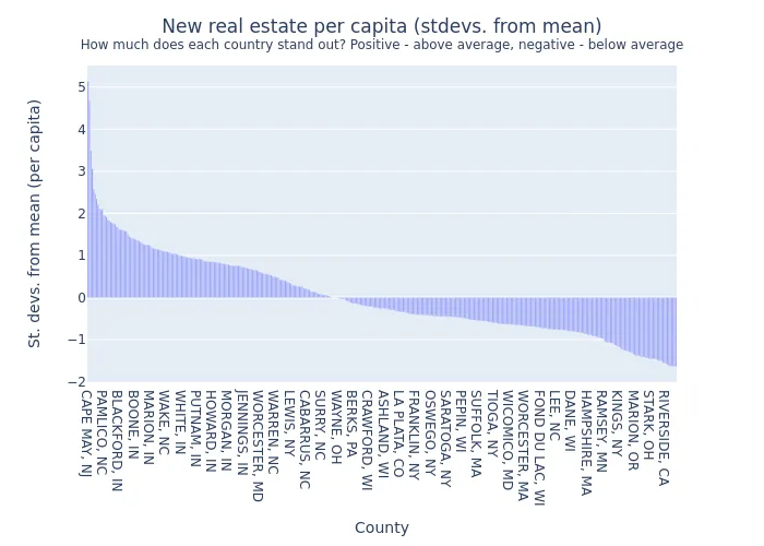

We can see that the spread is quite severe. Some counties have over two standard deviations more real estate developments than the mean value (per capita). Some other counties lag behind by having their per capita number below one standard deviation from the mean. Let us look into some outliers on both extremes to try getting some ideas for explanation.

What are top 10 counties we know of with highest per capita number of new real estate projects?

df_best_per_capita = df_counts_by_county.sort_values('per_capita', ascending=False).head(10)

fig = px.bar(df_best_per_capita, 
             x="county_state", 
             y="per_capita", 
             title="New real estate projects per capita<br><sub>Top 10 counties</sub>",
             labels=labels)
fig.write_image("top10_per_capita_by_county.png")
Image(filename="top10_per_capita_by_county.png")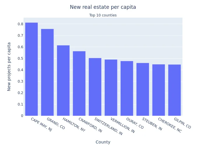

• Cape May County, NJ lays on southernmost part of New Jersey and is quite attractive to tourists, which also makes it attractive to real estate investors. This county is somewhat urbanized by coastal beach towns and has a moderate population density - largest in the top 10 list, but significantly lower than that in San Francisco.
• Grand County, CO is mostly rural place with low population density. The same applies to all entries on top 10 list except Cape May, NJ. It's probably not significant that these locations have high per capita amount of real estate developments, given that populations are small and per area amounts of new projects are below average. Unsurprisingly, lack of population means lack of NIMBYs.

What are the 10 counties with lowest per capita amounts of new real estate projects?

df_worst_per_capita = df_counts_by_county.sort_values('per_capita', ascending=True).head(10)
fig = px.bar(df_worst_per_capita,
             x="county_state",
             y="per_capita", 
             title="New real estate projects per capita<br><sub>Bottom 10 counties</sub>",
             labels=labels)
fig.write_image("worst10_per_capita_by_county.png")
Image(filename="worst10_per_capita_by_county.png")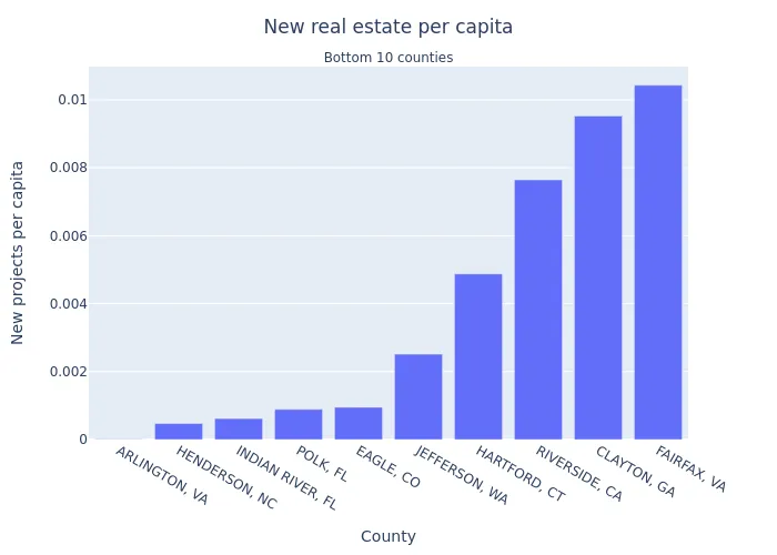

• Arlington, VA had only one sales record scraped during the bounty, so it's safe to say this is statistical anomaly.
• Most (but not all) of these areas are more urbanised with population density exceeding 200 people per square mile.
• Indian River County is on the eastern coast of Florida that is home to some fairly wealthy beach towns.
• Polk county, FL is fairly populous urban area within central Florida with a known resident opposition to new real estate projects.
• Riverside, CA is known to be difficult for real estate developers due to zoning and resident opposition.
• Clayton county, GA overlaps with Atlanta metropolitan area that is known for NIMBY activity.

Now, let us look into per-area numbers using the same kind of charts.

df_counts_by_county = df_counts_by_county.sort_values('per_area', ascending=False)
fig = px.bar(df_counts_by_county, 
             x='county_state', 
             y='per_area', 
             title="New real estate projects per area", 
             labels=labels)
fig.write_image("per_area_by_county.png")
Image(filename="per_area_by_county.png")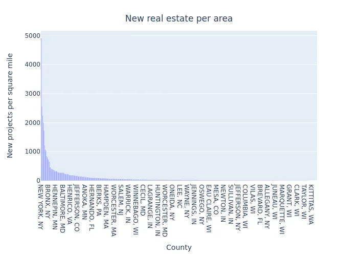

df_counts_by_county = df_counts_by_county.sort_values('per_area_stdevs_from_mean', ascending=False)
fig = px.bar(df_counts_by_county,
             x='county_state', 
             y='per_area_stdevs_from_mean', 
             title="New real estate projects per area (stdevs. from mean)<br><sup>How much does each country stand out in terms of new real estate projects?<br> Positive values mean above average, negative values mean below average</sup>", 
             labels=labels)
fig.write_image("per_area_stdevs_by_county.png")
Image(filename="per_area_stdevs_by_county.png")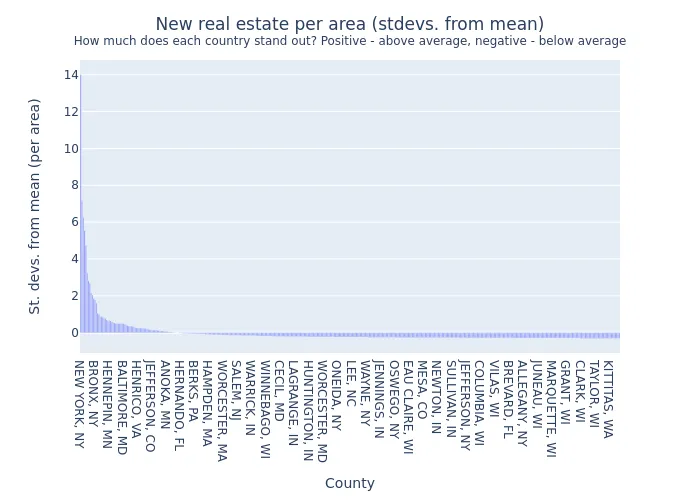

df_best_per_area = df_counts_by_county.sort_values('per_area', ascending=False).head(10)
fig = px.bar(df_best_per_area, 
             x="county_state", 
             y="per_area", 
             title="New real estate projects per capita<br><sub>Top 10 counties</sub>",
             labels=labels)
fig.write_image("top10_per_area_by_count.png")
Image(filename="top10_per_area_by_count.png")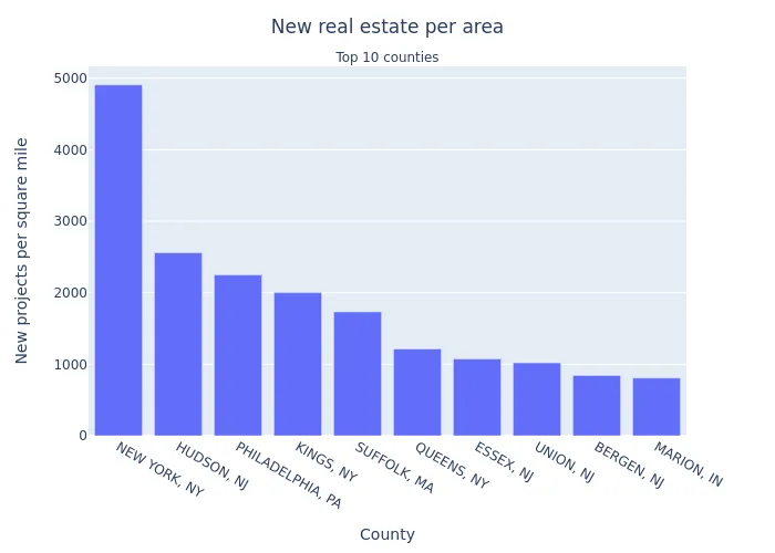

• A strong outlier here is New York County, which is probably unsurprising. Kings County (Brooklyn) and Queens County also have strong per-area values.
• Hudson, NJ is the most densely populated county in New Jersey. Some other counties of NJ are also represented.
• Philadelphia, PA is (was?) undergoing a real estate boom including some billion-dollar projects.
• Suffolk County, MA is of interest to investors and is now building some 10,000 new housing units.
• Distribution of per-area values has some positive outliers, but no negative outliers - after the initial drop off distance from the mean stays quite small.

Conclusion

What we have here is a good beginning. Although we were not able to conclusively pinpoint the easiest and the most difficult county for real estate developers to build new projects, we designed and implemented a way to do county-level outlier analysis that will remain applicable and grow in value once more data is sourced. We need more data. Even though the current data is fairly sparse and does not cover most of USA, some interesting outliers were found.

Stay tuned for the upcoming DoltHub data bounties!

Thanks to Rimantas for his guest contribution. Curious to discuss this article or guest contribute to our blog, come talk to us on Discord and ask for Tim.