
Introduction#
Dolt is Git for Data. It’s a SQL database that you can clone, fork, branch, and merge. Dolt’s SQL engine is go-mysql-server, and today we’re going to discuss how it implements join planning to make a query plan involving multiple tables as efficient as possible.
What’s join planning?#
When a query involves more than one table, there are many different ways to access those tables to get a correct result. But some ways are much faster than others! Choosing an order to access tables in and a strategy to assemble result rows is known as join planning. This is easiest to explain with an example.
Let’s create three tables to track the populations of cities and states, and the people who live in them. If you have Dolt installed (see instructions here), you can follow along.
% mkdir join-planning && cd join-planning
% dolt init
Successfully initialized dolt data repository.
% dolt sql
# Welcome to the DoltSQL shell.
# Statements must be terminated with ';'.
# "exit" or "quit" (or Ctrl-D) to exit.
join_planning> create table states (name varchar(100) primary key not null, population int unsigned);
join_planning> create table cities (name varchar(100) primary key not null, state varchar(100) not null, population int unsigned);
join_planning> create table people (name varchar(100) primary key not null, city varchar(100) not null);
Let’s say that we want a list of people named “John Smith” along with names and populations of the cities and states they live in. We would write a query like this:
select * from people p
    join cities c on p.city = c.name
    join states s on s.name = c.state
    where p.name = "John Smith";
There’s lots of ways that a query planner could execute this query. A
really bad way would be to look at every combination of every row from
all three tables and test each combination to see if it matches the
JOIN condition and WHERE clause. This is correct and valid, but
very expensive. If we say that the states, cities and people
tables contain S, C and P rows respectively, this query plan
(which is called a cross join), will result in S * C * P row
accesses and comparisons. It’s a bad idea.
There are simple tricks you can use to speed up query execution. Using
pushdown
optimization,
you can eliminate most of the accesses to the people table. Let’s
say that the number of “John Smiths” in the database is called J,
and it’s much smaller than P. Then using pushdown intelligently
reduces the cost of our access to S * C * J.
Until a few weeks ago, this was as good as Dolt could do on joins of three or more tables. For two tables, we would use an index if available. But for three, no luck. It made the product borderline unusable for a workload with this query pattern and a non-trivial data size.
This blog post is about how we optimized the join planner to generate more intelligent, efficient query plans for any number of tables. In today’s version of Dolt, that same query will generate the following query plan:
join_planning> explain select * from people p
    join cities c on p.city = c.name
    join states s on s.name = c.state
    where p.name = "John Smith";
+-------------------------------------------------------------+
| plan                                                        |
+-------------------------------------------------------------+
| IndexedJoin(p.city = c.name)                                |
|  ├─ Filter(p.name = "John Smith")                           |
|  │   └─ Projected table access on [name city]               |
|  │       └─ TableAlias(p)                                   |
|  │           └─ Indexed table access on index [people.name] |
|  │               └─ Exchange(parallelism=16)                |
|  │                   └─ Table(people)                       |
|  └─ IndexedJoin(s.name = c.state)                           |
|      ├─ TableAlias(c)                                       |
|      │   └─ IndexedTableAccess(cities on [cities.name])     |
|      └─ TableAlias(s)                                       |
|          └─ IndexedTableAccess(states on [states.name])     |
+-------------------------------------------------------------+
The plan starts with an indexed access on the name column of
people to find all the John Smiths. Then for each row, it uses a
primary key index to look up the city. Then for each city, it uses
another primary key to look up the state. In all, this leads to a
total query cost of J * 3.
Is that… a lot?#

Using some real numbers to drive this home: let’s use the US and say
that there are 330,000,000 people rows, 20,000 cities rows, and 52
states rows (we didn’t forget you, DC and Puerto Rico). A cross join
query plan would access a number of rows equal to the product of these
numbers, which is roughly 343 trillion accesses. It’s a big
number. Your query isn’t going to complete.
There are about 48,000 people named John Smith in the US. So using pushdown optimization gets us down to about 50 billion row accesses. This is a lot better than before, but still terrible. The query isn’t returning.
Using both pushdown to the people table and indexed accesses to
cities and states, on the other hand, limits the query execution
to only 48,000 accesses to the people table, then 1 access to each of
the cities and states table for each of these rows. That’s 3 * 48,000, or 144,000 table accesses total.
| Join plan | Number of rows accessed |
|---|---|
| Cross join | 343 * 10^12 |
| Cross join with pushdown | 50 * 10^9 |
| Pushdown and indexed access | 144 * 10^3 |
Unlike in the pushdown blog, I won’t bother to spell out the percentage savings. We’re looking at 4 decimal orders of magnitude improvement for the first optimization, then another 5 for the second. It’s the difference between Dolt being a usable query engine or a bad space heater.
How does it work?#
To assemble an efficient query plan, you have to start by by answering one really important question:
What order should we access the tables in?
This really makes all the difference. In the example above, a table
access order of people > cities > states lets us use the primary key
index on the latter two tables. If we instead chose the order states > cities > people,
we can’t use the information from earlier tables
to reduce the number of lookups into later tables, giving us a cross join.
There are a lot of interesting details to get wrong, but to get table order right you can use some pretty simple heuristics.
- What index could I use to access this table? Are those columns part of a join condition?
- Are required columns available to use as a key? Did the other tables in the join condition precede this one?
- How many rows are in this table if I need to do a full table scan?
- Is this a
LEFTorRIGHTjoin, and if so, is this table on the side of the join that requires it to come first?
We’ll come back to the actual implementation of the table ordering algorithm later. For now let’s assume its existence, and it tells us which order to access tables in. How do we build a join plan with that access order?
Join plans are not isomorphic#
In go-mysql-server,
query plans are organized in a tree of Node objects. As of now, all
nodes have at most two children, making the query plan a binary-ish
tree. A Join node knows how to get a row from its left child, then
iterate over its right child looking for matches on the join
condition. When the right child iterator is out of rows, it gets the
next row from its left child. Eventually it runs out of rows in the
left child and returns io.EOF from its iterator.
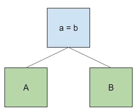
Like everything else, this is easiest to visualize with some examples. For all of these, we’ll use one-letter table names with single columns that match the table name. Here’s a simple join between two tables A and B:
select * from A join B on a = b;A naive query plan looks like this:
As we add additional tables to the join, they become the new root of the tree, with the original subtree as the left child.
select * from A join B on a = b join C on b = c;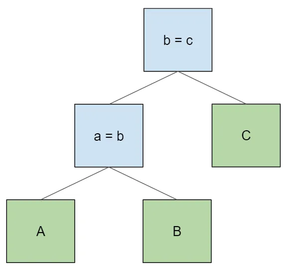
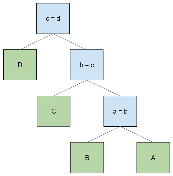
select * from A join B on a = b join C on b = c join D on c = d;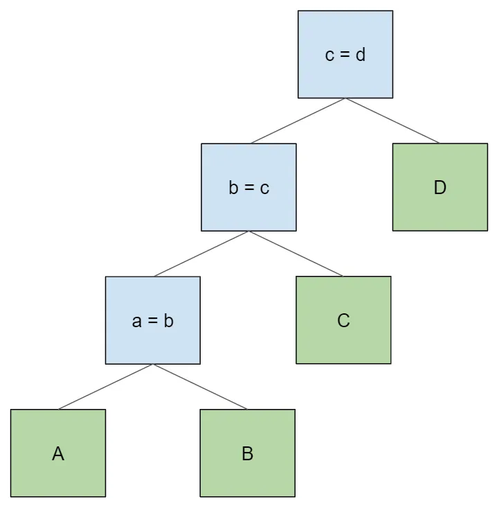
Let’s examine this last example more closely. What happens when we
open an iterator on the root Node of the query? It opens an iterator
on its left child, which in turn opens an iterator on its left child,
and so on. Each node, after accessing a row from its left child, then
attempts to find a matching row from its right child. We end up with
the table access order the same as in the lexical query: A > B > C > D.
Let’s trace through the execution of a single row in the result set.
- The join node
a = bgets a row fromA. Then it iterates through the rows ofBlooking for rows that match the join conditiona = b. When it finds such a row, it returns it. - The node
b = ctakes the row from its left child, which is a concatenation of rows from tablesAandB. It then iterates over its right child, the rows ofC, looking for rows that match the join conditionb = c. When it finds such a row, it returns it. - The node
c = dtakes the row from its left child, which is a concatenation of rows fromAandBandC, in that order. It then attempts to match rows from its right child,D, just as above.
Importantly, there are sometimes many possible binary trees that can implement the above logic to yield a correct result for any given table access order. The tree construction algorithm above, where we keep shoving a sub-tree down to the left child of a new join node, is just what the parser gives us by default because it’s left associative. But we can draw other trees that give the same results. For example, here’s a balanced join tree:
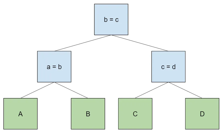
Like the original, this produces a table access order of A > B > C > D. If we wanted to access the tables in the opposite order, we could
simply flip the left and right children of every node in the original
tree like so:
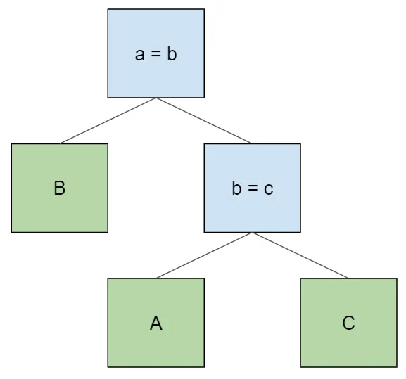
Again, there are sometimes many possible join trees for a given table
ordering. But they all have one thing in common: their join conditions
refer to tables that can be found in their left and right
children. Otherwise, the node cannot evaluate its join condition. For
example, let’s say that we are querying three tables and want to
access them in the order B > A > C. This is an invalid join plan
with that table ordering:
This plan is invalid because the node b = c doesn’t have table B
as a descendant, so it cannot evaluate its join condition. We can’t
get around this issue by just swapping the join conditions, either:
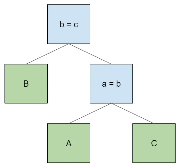
The lower join condition still isn’t satisfied, this time because it
needs table B and doesn’t have it as a descendant. In order to get
the order B > A > C and still satisfy the join conditions, we need
to produce this tree instead:
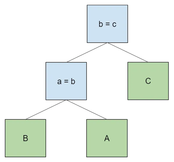
Join search#
We can use the above insights about constructing a join tree to come up with a general algorithm for doing so. It’s a constraint solving / search problem, and in the source code I call it join search.
- Choose a join condition from the set of available join conditions to begin with.
- Construct all possible left subtrees for this join condition recursively, using the remaining tables and join conditions.
- Check each potential left subtree for validity: the tables must be in order, and the join conditions must be satisfied. If a subtree is not valid, discard it and examine the next one.
- Construct all possible right subtrees for this join condition recursively, using the remaining tables and join conditions (making sure to remove from consideration all tables and join conditions used by the left subtree). Again discard subtrees that aren’t valid.
- If you can’t find a valid left or right subtree, give up and go back to step one, choosing a new join condition to begin with.
Like most things in this tech blog series, the idea is relatively
simple but there are many small details to screw up. Because the
Node objects are pretty cumbersome to work with, I created a
simplified type to represent the join tree during search:
// A joinSearchNode is a simplified type representing a join tree node, which is either an internal node (a join) or a
// leaf node (a table). The top level node in a join tree is always an internal node. Every internal node has both a
// left and a right child.
type joinSearchNode struct {
    table    string            // empty if this is an internal node
    joinCond *joinCond         // nil if this is a leaf node
    parent   *joinSearchNode   // nil if this is the root node
    left     *joinSearchNode   // nil if this is a leaf node
    right    *joinSearchNode   // nil if this is a leaf node
    params   *joinSearchParams // search params that assembled this node
}
Besides the normal tree structure, this type also tracks a parent pointer (to make it easier to walk from the root to validate table ordering rules) and search params to track which tables and join conditions are available for use.
Here’s a portion of the searchJoins function that implements this
algorithm. The full code is linked above.
func searchJoins(parent *joinSearchNode, params *joinSearchParams) []*joinSearchNode {
    // Our goal is to construct all possible child nodes for the parent given. Every permutation of a legal subtree should
    // go into this list.
    children := make([]*joinSearchNode, 0)

    // <snipped code appending tables to the list of children>

    for i, cond := range params.joinConds {
        if params.joinCondIndexUsed(i) {
            continue
        }

        paramsCopy := params.copy()
        paramsCopy.usedJoinCondsIndexes = append(paramsCopy.usedJoinCondsIndexes, i)

        candidate := &joinSearchNode{
            joinCond: cond,
            parent:   parent,
            params:   paramsCopy,
        }

        // For each of the left and right branch, find all possible children, add all valid subtrees to the list
        candidate = candidate.targetLeft()
        leftChildren := searchJoins(candidate, paramsCopy)

        // pay attention to variable shadowing in this block
        for _, left := range leftChildren {
            if !isValidJoinSubTree(left) {
                continue
            }
            candidate := candidate.withChild(left).targetRight()
            candidate.params = candidate.accumulateAllUsed()
            rightChildren := searchJoins(candidate, paramsCopy)
            for _, right := range rightChildren {
                if !isValidJoinSubTree(right) {
                    continue
                }
                candidate := candidate.withChild(right)
                if isValidJoinSubTree(candidate) {
                    children = append(children, candidate)
                }
            }
        }
    }

    return children
}
Plumbing key information through#
Now that we have a table order and a join plan that implements that order, we need a way to get key information to later tables in the plan. The whole reason that we ordered tables was to make it possible to use indexed lookups on every table but the first. For each of these tables, we want to pass the concatention of the rows from all earlier tables in the join, so that we can use this information to construct a lookup key for an index.
Consider this four-table join plan. For each edge in the tree, we’ll label the edge with the tables that the child node need access to in order to look up key information in any table to its left.
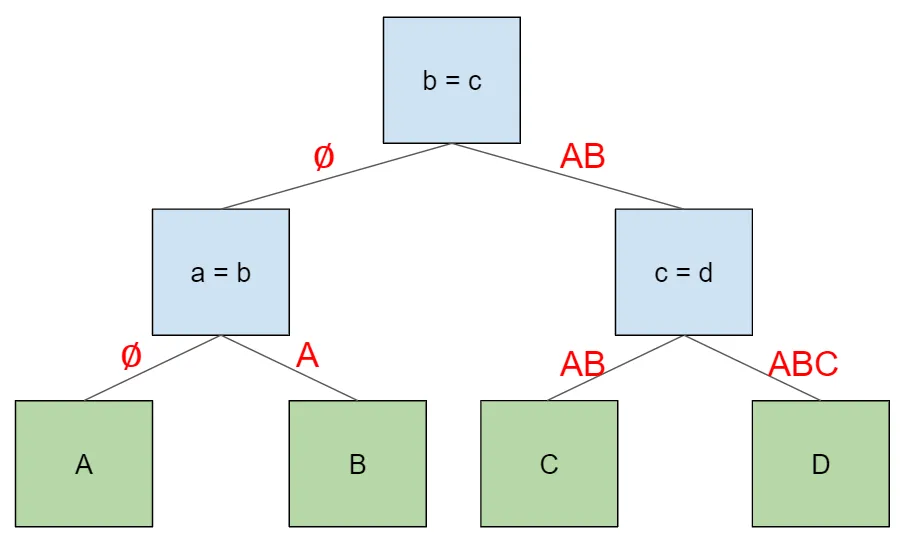
Each join node will supply its left-hand child with the row it
received (empty in the case of the root node). Then it will supply its
right-hand child the concatenation of this row and the row from the
left-hand child. This amounts to an in-order walk of the tree, which
will visit the tables in the order we specified in the
beginning. First, the root node traverses left with an empty row. The
same thing happens in the first child node (a = b). When this child
node traverses to the right, it supplies the row from its left-hand
child, A. Then the root node traverses right, and supplies the row
from its left child, which corresponds to AB. The same thing happens
in the final node (c = d), where the final right-hand child gets a
row formed by the concatenation of its parent row (AB) and its
left-hand child (C).
Unlike most of the rest of engine analysis, we can’t do this transformation of the tree bottom up. It’s fundamentally an in-order walk, so we have to do it top down with a custom function. Here’s the interesting portion of it (with some small edits, like removing error handling boilerplate and simplifying the return type).
func replaceTableAccessWithIndexedAccess(
    node sql.Node,
    schema sql.Schema,
    scope *Scope,
    joinIndexes joinIndexesByTable,
    exprAliases ExprAliases,
    tableAliases TableAliases,
) sql.Node {

    switch node := node.(type) {
    case *plan.TableAlias, *plan.ResolvedTable:
        // If the available schema makes an index on this table possible, use it, replacing the table with indexed access
        indexes := joinIndexes[node.(sql.Nameable).Name()]
        indexToApply := indexes.getUsableIndex(schema)
        if indexToApply == nil {
            return node
        }

        node, err := plan.TransformUp(node, func(node sql.Node) (sql.Node, error) {
            switch node := node.(type) {
            case *plan.ResolvedTable:
                if _, ok := node.Table.(sql.IndexAddressableTable); !ok {
                    return node
                }

                keyExprs := createIndexLookupKeyExpression(indexToApply, exprAliases, tableAliases)
                keyExprs, err := FixFieldIndexesOnExpressions(scope, schema, keyExprs...)

                return plan.NewIndexedTableAccess(node, indexToApply.index, keyExprs)
            default:
                return node
            }
        })

        return node
    case *plan.IndexedJoin:
        // Recurse the down the left side with the input schema
        left, replacedLeft, err := replaceTableAccessWithIndexedAccess(node.Left(), schema, scope, joinIndexes, exprAliases, tableAliases)

       // then the right side, appending the schema from the left
       right, replacedRight, err := replaceTableAccessWithIndexedAccess(node.Right(), append(schema, left.Schema()...), scope, joinIndexes, exprAliases, tableAliases)

       // the condition's field indexes might need adjusting if the order of tables changed
       cond, err := FixFieldIndexes(scope, append(schema, append(left.Schema(), right.Schema()...)...), node.Cond)
       return plan.NewIndexedJoin(left, right, node.JoinType(), cond)
   default:
       // Other node types
       newChild, replaced, err := replaceTableAccessWithIndexedAccess(node.Child, schema, scope, joinIndexes, exprAliases, tableAliases)
       return node.WithChildren(newChild)
   }
}
Back to the beginning: choosing a table order#
Now we’re back to where we started: how do we decide which order tables should be accessed in? This part is relatively easy now that we’ve put all the other pieces together. To determine an optimal ordering, all we need is a set of the join conditions with index information attached. Then the function is pretty simple to write:
// orderTables returns an access order for the tables provided, attempting to minimize total query cost
func orderTables(tables []NameableNode, tablesByName map[string]NameableNode, joinIndexes joinIndexesByTable) []string {
    tableNames := make([]string, len(tablesByName))
    indexes := make([]int, len(tablesByName))
    for i, table := range tables {
        tableNames[i] = strings.ToLower(table.Name())
        indexes[i] = i
    }

    // generate all permutations of table order
    accessOrders := permutations(indexes)
    lowestCost := int64(math.MaxInt64)
    lowestCostIdx := 0
    for i, accessOrder := range accessOrders {
        cost := estimateTableOrderCost(tableNames, tablesByName, accessOrder, joinIndexes, lowestCost)
        if cost < lowestCost {
            lowestCost = cost
            lowestCostIdx = i
        }
    }

    cheapestOrder := make([]string, len(tableNames))
    for i, j := range accessOrders[lowestCostIdx] {
        cheapestOrder[i] = tableNames[j]
    }

    return cheapestOrder
}
But this is burying the lede a bit. Estimating the cost of a table ordering is the juicy part.
// Estimates the cost of the table ordering given. Lower numbers are better. Bails out and returns cost so far if cost
// exceeds lowest found so far. We could do this better if we had table and key statistics.
func estimateTableOrderCost(
	tables []string,
	tableNodes map[string]NameableNode,
	accessOrder []int,
	joinIndexes joinIndexesByTable,
	lowestCost int64,
) int64 {
	cost := int64(1)
	var availableSchemaForKeys sql.Schema
	for i, idx := range accessOrder {
		if cost >= lowestCost {
			return cost
		}

		table := tables[idx]
		availableSchemaForKeys = append(availableSchemaForKeys, tableNodes[table].Schema()...)
		indexes := joinIndexes[table]

		// If this table is part of a left or a right join, assert that tables are in the correct order. No table
		// referenced in the join condition can precede this one in that case.
		for _, idx := range indexes {
			if (idx.joinType == plan.JoinTypeLeft && idx.joinPosition == plan.JoinTypeLeft) ||
				(idx.joinType == plan.JoinTypeRight && idx.joinPosition == plan.JoinTypeRight) {
				for j := 0; j < i; j++ {
					otherTable := tables[accessOrder[j]]
					if colsIncludeTable(idx.comparandCols, otherTable) {
						return math.MaxInt64
					}
				}
			}
		}

		if i == 0 || indexes.getUsableIndex(availableSchemaForKeys) == nil {
			// TODO: estimate number of rows in table
			cost *= 1000
		} else {
			// TODO: estimate number of rows from index lookup based on cardinality
			cost += 1
		}
	}

	return cost
}
The engine doesn’t have table statistics yet, so for the time being
we’re treating any full table scan as a factor of 1000, and any
indexed lookup as constant cost. And we rule out join plans that
access the primary tables in LEFT or RIGHT joins incorrectly by
making them maximally expensive.
Future work#
In our discussion so far, we concentrated on table ordering and the use of index lookups. This is an important aspect to join planning, but not the only one. We also need to consider different join strategies other than simple nested loop joins, such as the hash joins that SQL Server makes such extensive use of. For certain table sizes, it’s much faster to load a table result set in memory and hash join it to the rest of the query than to do N indexed lookups into it. But this is work for another day.
Conclusion#
It’s been almost a year since we announced support for indexed joins for two tables. We’ve come a long way since then, rewriting large parts of the engine and adding tons of features. This latest improvement, indexed joins for any number of tables, was the most difficult addition I’ve made to the engine yet. It took a lot of careful thought and analysis, tons of experimentation and false starts, and a crazy amount of tests.
But it’s also the most satisfying addition I’ve made. It takes the query engine from unusably slow to actually functional for a lot of customers. It makes the product seem like a real database, not just a cool toy. And it actually makes use of the hard parts of my computer science education, unlike nearly all my professional software experience. That’s a good feeling.
Dolt is a great tool to learn how to use SQL, now with non-terrible performance on queries with three or more tables. Install Dolt today to try it out. Or if you aren’t ready to download the tool or just want to ask questions, come chat with us on Discord. We’re always happy to hear from new customers!