
Introduction#
In the past we have blogged about the IRS Sources of Income (SOI) data that we harvested and published as a Dolt database. We presented a compelling visualization that was relatively straightforward to create using that database. It was straightforward to create because of the work that went into transforming disparate and unruly files to a coherently presented database. Recently we highlighted a dataset of USPS Crosswalk mappings that are widely used into academic and commercial settings to traverse between ZIP code and other geographic statistical entities, for example counties. They are also available as a Dolt database. Finally just today we published US Census Bureau population estimates by county, indexed on FIPS code going back to 2010.
One of the most impressive features of using Dolt and DoltHub together is how elegant they make acquiring these datasets in your local environment. There is no need to sign up, and we aren’t tying you to a compute environment we will try and charge you for. They simply enable distribution of datasets along with a SQL interface. Dolt runs wherever you need it to run. Users can skip downloading, parsing, and cleaning collections of files, and begin analyzing the data immediately.
In this post we show how these features make it easy to combine a specifically interesting dataset, the IRS SOI data, with generally useful datasets, the USPS Crosswalk data and county level population estimates, to essentially toggle the spatial resolution of the IRS data. We conclude by advocating for the concept of a data dependency delivered as a “drop in” resource. The benefit of this model is for companies and individuals that depend on data, but do not see at as a core competency, to focus on what they do best. This is very much how open source software works.
Requirements#
To work through this locally you will need to get a copy of Dolt, which on *nix systems can be done with a single command, and we have documentation on the full range of installation options here:
$ sudo bash -c 'curl -L https://github.com/dolthub/dolt/releases/latest/download/install.sh | sudo bash'For the analysis component, you will need Doltpy, which has all other libraries imported in the sample code as a dependency. It’s available on PyPi:
$ pip install doltpyFor the visualization you will need several Python libraries, but they can easily be installed as follows:
pip install plotly plotly-geo geopandas==0.3.0 pyshp==1.2.10Let’s move onto to acquiring data.
Acquiring data#
Acquiring data with Dolt is easy. Let’s set up a home for our analysis:
$ mkdir -p ~/irs-analysis/dolt-dbs && cd irs-analysis/dolt-dbs
$ dolt clone dolthub/irs-soi
cloning https://doltremoteapi.dolthub.com/dolthub/irs-soi
291,637 of 291,637 chunks complete. 0 chunks being downloaded currently.
$ dolt clone dolthub/usps-crosswalk-data
cloning https://doltremoteapi.dolthub.com/dolthub/usps-crosswalk-data
210,458 of 210,458 chunks complete. 0 chunks being downloaded currently.
$  dolt clone dolthub/census-population-estimates
cloning https://doltremoteapi.dolthub.com/dolthub/census-population-estimates
82 of 82 chunks complete. 0 chunks being downloaded currently.
We now have two Dolt databases in ~/irs-analysis/dolt-dbs, and we can launch the Dolt SQL shell in with the --multi-db-dir switch to make load them both into our SQL environment:
$ ls -ltr
total 0
drwxr-xr-x  12 oscarbatori  staff  384 Jul 23 18:07 irs-soi
drwxr-xr-x   6 oscarbatori  staff  192 Jul 23 21:11 usps-crosswalk-data
$ dolt sql --multi-db-dir .
~/Documents/irs-analysis/dolt-dbs|>>  dolt sql --multi-db-dir .
# Welcome to the DoltSQL shell.
# Statements must be terminated with ';'.
# "exit" or "quit" (or Ctrl-D) to exit.
> show databases;
+-----------------------------+
| Database                    |
+-----------------------------+
| census_population_estimates |
| information_schema          |
| irs_soi                     |
| usps_crosswalk_data         |
+-----------------------------+
We have now acquired two datasets, both maintained by DoltHub. We can use dolt pull to subscribe to changes to the datasets, making any derivative analysis we create “live.”
The Data#
We will be working with adjusted gross income by ZIP code, and then using the USPS Crosswalk data and county population estimate to translate that to county level per capita income. This works because the USPS publishes mappings from ZIP codes to various geographical statistical entities identified by FIPS code, mappings that we completely capture (across time and mapping pairs). The data includes “ratios” of residential and business addresses for pairings that are not one to one. For example a ZIP code and straddle county lines, and vice versa, and so these ratios provide a mechanism for us approximate how much of a given aggregate to apportion when we perform the mapping.
Let’s take a peek at the data to see how it looks in practice:
> use irs_soi;
Database changed
irs_soi> select * from agi_by_zip limit 5;
+------+-------+-------+----------+--------+
| year | state | zip   | category | agi    |
+------+-------+-------+----------+--------+
| 2011 | AK    | 99501 | 1        | 43489  |
| 2011 | AK    | 99501 | 2        | 101801 |
| 2011 | AK    | 99501 | 3        | 69202  |
| 2011 | AK    | 99501 | 4        | 53289  |
| 2011 | AK    | 99501 | 5        | 103854 |
+------+-------+-------+----------+--------+
irs_soi> use usps_crosswalk_data;
Database changed
usps_crosswalk_data> select * from zip_county limit 10;
+-------+--------+-----------+-----------+-----------+-----------+-------+------+
| zip   | county | res_ratio | bus_ratio | tot_ratio | oth_ratio | month | year |
+-------+--------+-----------+-----------+-----------+-----------+-------+------+
| 00501 | 36103  | 0         | 1         | 1         | 0         | 3     | 2010 |
| 00501 | 36103  | 0         | 1         | 1         | 0         | 3     | 2011 |
| 00501 | 36103  | 0         | 1         | 1         | 0         | 3     | 2012 |
| 00501 | 36103  | 0         | 1         | 1         | 0         | 3     | 2013 |
| 00501 | 36103  | 0         | 1         | 1         | 0         | 3     | 2014 |
+-------+--------+-----------+-----------+-----------+-----------+-------+------+
> use census_population_estimates;
Database changed
census_population_estimates> select * from county_population_estimates limit 5;
+-------------------------+-------+------+------------+
| county                  | fips  | year | population |
+-------------------------+-------+------+------------+
| Autauga County, Alabama | 01001 | 2010 | 54773      |
| Autauga County, Alabama | 01001 | 2011 | 55227      |
| Autauga County, Alabama | 01001 | 2012 | 54954      |
| Autauga County, Alabama | 01001 | 2013 | 54727      |
| Autauga County, Alabama | 01001 | 2014 | 54893      |
+-------------------------+-------+------+------------+
We can see here a bunch of ZIP codes that are completely contained within counties. These ZIP codes contain only business addresses. That’s not always the cade. Let’s step into Python and do some analysis.
Analysis#
We saw earlier how easy it was to acquire the data from DoltHub using Dolt. The USPS Crosswalk dataset took around 450 files to build, each of them Excel files. So running a single command was a pretty big time saving, even over the narrow subset of the data we are interested in, around 50 files. Loading them into Dolt also required removing some corrupt data, so that work is now embedded in the database, and amortized over everyone that takes advantage of it.
This simple acquisition model is only fraction of the benefit of acquiring data via Dolt and DoltHub. The balance comes from the SQL interface that arrives with the data. We don’t need to parse files, we can just use SQL’s elegant declarative syntax to describe the data we are interested in, and then let the query engine deliver it to our preferred interface, in this case Python.
The goal of our analysis is to translate ZIP code level income data to the county level, so let’s grab each dataset, and then combine them:
from doltpy.core.dolt import Dolt, ServerConfig
import doltpy.core.read as dcr
import sqlalchemy
from retry import retry


def get_data(irs_repo_path: str, multi_db_dir: str):
    repo = Dolt(irs_repo_path, server_config=ServerConfig(multi_db_dir=multi_db_dir))
    start_server(repo)

    with repo.get_engine().connect() as conn:
        conn.execute('USE irs_soi')
        query = '''
            SELECT
                `year`,
                `state`,
                `zip`,
                SUM(`agi`) as `agi`
            FROM
                `agi_by_zip`
            WHERE
                `zip` != '99999'
            GROUP BY
                `year`,
                `state`,
                `zip`
        '''
        agi_data = dcr.pandas_read_sql(query, conn)

    with repo.get_engine().connect() as conn:
        conn.execute('USE usps_crosswalk_data')
        query = '''
            SELECT
                `year`,
                `zip`,
                `res_ratio` as `ratio`,
                `county`
            FROM
                `zip_county`
            WHERE
                `month` = 3
                AND `year` >= 2011
                AND `year` <= 2017;
        '''
        crosswalk_data = dcr.pandas_read_sql(query, conn)

    with repo.get_engine().connect() as conn:
        conn.execute('USE census_population_estimates')
        query = '''
            SELECT
                `fips` as `county`,
                `year`,
                `population`
            FROM
                `county_population_estimates`
            WHERE
                `year` >= 2011
                AND `year` <= 2017;
                        '''
        county_population_data = dcr.pandas_read_sql(query, conn)

    return combine_data(crosswalk_data, agi_data, county_population_data)


@retry(exceptions=(sqlalchemy.exc.OperationalError, sqlalchemy.exc.DatabaseError), delay=2, tries=10)
def start_server(repo: Dolt):
    '''
    Verify that the server has started by ensuring we can connect to it.
    '''
    repo.sql_server()
    with repo.get_engine().connect() as conn:
        conn.execute('show databases')
By breaking out the combiner into a separate function we separate the simplicity of reading from Dolt from the complexity of our analysis, which though itself relatively simple, necessitates some domain knowledge of the data at hand. This function left joins the ZIP to county mappings to the ZIP code level adjusted gross income values, along with “residential ratio”. For a given pairing of ZIP code and county the residential ratio is the fraction of residential addresses in that ZIP code that reside in that county. This gives us an approximate mechanism for apportioning ZIP code level incomes totals across counties when a ZIP code straddles more than a single county. We can immediately check how common this is, again highlighting the value of being able to immediately explore our data without writing programs to do so:
> use usps_crosswalk_data;
Database changed
usps_crosswalk_data> select count(*) from zip_county where res_ratio in (1, 0) and  month = 3 and year = 2020;
+----------+
| COUNT(*) |
+----------+
| 28697    |
+----------+
usps_crosswalk_data> select count(*) from zip_county where month = 3 and year = 2020;
+----------+
| COUNT(*) |
+----------+
| 54181    |
+----------+
In just under half of cases a ZIP code straddles a county line, something I have to admit I was personally quite surprised by. This underscores the importance of accounting for this effect. After joining the ZIP to county mappings to the ZIP level AGI data we compute the dollar contribution of the ZIP code to the county by multiplying the adjusted gross income by the residential ratio value, and then aggregate at the county level to get county level totals:
import pandas as pd

def combine_data(zip_to_county_crosswalk: pd.DataFrame,
                 agi_by_zip: pd.DataFrame,
                 county_populations: pd.DataFrame):
    index = ['year', 'zip']
    indexed_agi, indexed_crosswalk = agi_by_zip.set_index(index), zip_to_county_crosswalk.set_index(index)
    combined = indexed_agi.join(indexed_crosswalk, how='left')
    ratiod = combined.assign(agi=combined['agi'] * combined['ratio']).reset_index().dropna(subset=['county'])
    by_county = ratiod.groupby(['year', 'county', 'state'])[['agi']].sum().reset_index()
    by_county_with_pop = by_county.set_index(['year', 'county']).join(county_populations.set_index(['year', 'county']),
                                                                      how='left')
    by_county_with_pop.loc[:, 'per_capita_agi'] = by_county_with_pop['agi'] / by_county_with_pop['population']
    return by_county_with_pop.dropna(subset=['population'])
There is some final cleanup pertaining to how Pandas interprets integer values as floats, but this is merely for presentation. Note that we wrote very little code here, the simplicity and guarantees provided by the use of a database for store data, rather than loosely defined formats such as CSV, enabled us to quickly proceed to the meat of our analysis.
Visualization#
We use Plotly for our visualization. It’s an open source charting library with some interesting features for plotting geogrpahic data. The code for the setup is relatively straightforward:
from irs_analysis.scratch import get_data
from plotly import figure_factory as ff
import numpy as np
# Note we have to fix one of our Dolt directories as the base for Dolt the
# second parameter is the parent directory for multi-db mode to query across
# multiple Dolt databases
data = get_data('~/irs-analysis/dolt-dbs', 'irs-analysis/dolt-dbs')
fips = data[data['year'] == 2017]['county'].tolist()
values = data[data['year'] == 2017]['per_capita_agi'].tolist()

colorscale = [
    "#85bcdb", "#6baed6", "#57a0ce", "#4292c6", "#3082be", "#2171b5", "#1361a9",
    "#08519c", "#0b4083", "#08306b"
]

fig = ff.create_choropleth(
    fips=fips,
    values=values,
    scope=['usa'],
    binning_endpoints=list(np.linspace(1, max(values), len(colorscale) - 1)),
    colorscale=colorscale,
    show_state_data=False,
    show_hover=True,
    asp=2.9,
    title_text='2017 Per capita AGI',
    legend_title='Per capita AGI'
)
fig.layout.template = None
fig.show()
You can read more about producing “choropleth” visualizations on Plotly’s documentation. Here is the output:
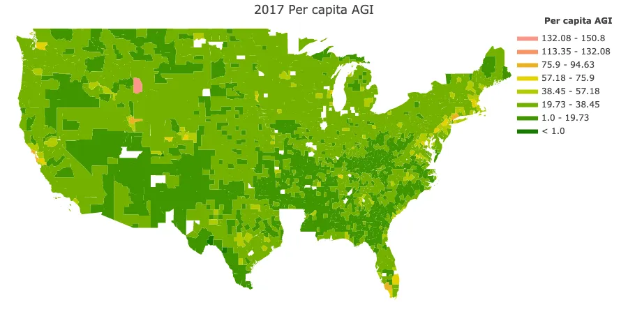
We can see darker areas around wealth coastal cities, but then also small counties, such as Teton, WY, which is an extremely wealthy county. It happens to be where Jackson is located, of Jackson Hole fame. It seems that at the county level smaller counties that amount to “wealthy enclaves” stomp the effects of larger wealthy areas, such as Manhattan (New York County) which are diluted by possessing a degree of economic diversity.
Data as a Resource#
In a recent blogpost announcing the USPS Crosswalk dataset on DoltHub, we advanced the notion of a dataset as a “drop in resource” analogous to the way we might think of open source software. Dolt took significant design cues from Git, particularly its core data structure and distribution model, and the goal of doing so was precisely to enable organizations to drop data dependencies straight into the production infrastructure. CSV, JSON, and other file formats, are fine ways to distribute data, but they don’t constitute a robust dependency mechanism. We want to organizations and researchers to be able to depend on generally useful datasets with minimal cognitive load precisely so they can focus more deeply on their core competencies.
This analysis highlighted a concrete example of that. We combined a specifically interesting dataset, adjusted gross income at the ZIP code level, with a generally useful dataset, USPS crosswalk data for mapping ZIP codes to counties. This crosswalk data could be useful anywhere that researchers are looking to traverse between ZIP codes and other statistical geographic areas identified by a FIPs code. Many forms of analysis, including financial models, academic research, marketing, and more, depend on the ability to translate between geographic locales. Users should not have to download and parse those files, or pay for them. They should just acquire that data as a coherent database, and then subscribe to updates from the upstream. This model virtually eliminated friction in distribution and collaboration for source code, enabling companies to outsource pieces of their core infrastructure that didn’t represent a core competency to community efforts. We believe something similar should happen for generically useful datasets.
Conclusion#
Here we used a specific example of how to take advantage of generally useful datasets on DoltHub to enhance an existing dataset of interest, also on DoltHub, though it need not be. Normally the more specific dataset will be private, perhaps a proprietary one owned by an organization or researcher.
The wider goal of this post was to highlight the value of a distribution model inspired by Git and SQL databases that aims to empower the user to immediately get value from acquired data by elevating the quality of the data they acquire and providing a deeply familiar interface for exploring and querying it.
If you found this interesting, sign up for DoltHub and start exploring.